Propensity Modelling - Using h2o and DALEX to Estimate the Likelihood of Purchasing a Financial Product - Data Preparation and Exploratory Data Analysis
In this day and age, a business that leverages data to understand the drivers of its customers’ behaviour has a true competitive advantage. Organisations can dramatically improve their performance in the market by analysing customer level data in an effective way and focus their efforts towards those that are more likely to engage.
One trialled and tested approach to tease out this type of insight is Propensity Modelling, which combines information such as a customers’ demographics (age, race, religion, gender, family size, ethnicity, income, education level), psycho-graphic (social class, lifestyle and personality characteristics), engagement (emails opened, emails clicked, searches on mobile app, webpage dwell time, etc.), user experience (customer service phone and email wait times, number of refunds, average shipping times), and user behaviour (purchase value on different time-scales, number of days since most recent purchase, time between offer and conversion, etc.) to estimate the likelihood of a certain customer profile to performing a certain type of behaviour (e.g. the purchase of a product).
Once you understand the probability of a certain customer to interact with your brand, buy a product or sign up for a service, you can use this information to create scenarios, be it minimising marketing expenditure, maximising acquisition targets, and optimise email send frequency or depth of discount.
Project Structure
In this project I’m analysing the results of a bank direct marketing campaign to sell term deposits in order to identify what type of customer is more likely to respond. The marketing campaigns were based on phone calls and more than one contact to the same client was required at times.
First, I am going to carry out an extensive data exploration and use the results and insights to prepare the data for analysis.
Then, I’m estimating a number of models and assess their performance and fit to the data using a model-agnostic methodology that enables to compare traditional “glass-box” models and “black-box” models.
Last, I’ll fit one final model that combines findings from the exploratory analysis and insight from models’ selection and use it to run a revenue optimisation.
The data
library(tidyverse)
library(data.table)
library(skimr)
library(correlationfunnel)
library(GGally)
library(ggmosaic)
library(knitr)
The Data is the Portuguese Bank Marketing set from the UCI Machine Learning Repository and describes the direct marketing campaigns carried out by a Portuguese banking institution aimed at selling term deposits/certificate of deposits to their customers. The marketing campaigns were based on phone calls to potential buyers from May 2008 to November 2010.
Of the four variants of the datasets available on the UCI repository, I’ve chosen the bank-additional-full.csv which contains 41,188 examples with 21 different variables (10 continuous, 10 categorical plus the target variable). A full description of the variables is provided in the appendix.
In particular, the target subscribed is a binary response variable indicating whether the client subscribed (‘Yes’ or numeric value 1) to a term deposit or not (‘No’ or numeric value 0), which make this a binary classification problem.
Loading data and initial inspection
The data I’m using ( bank-direct-marketing.csv) is a modified version of the full set mentioned earlier and can be found on my GitHub profile. As it contains lots of double quotation marks, some manipulation is required to get into a usable format.
First, I load each row into one string
data_raw <-
data.table::fread(
file = "../01_data/bank_direct_marketing_modified.csv",
# use character NOT present in data so each row collapses to a string
sep = '~',
quote = '',
# include headers as first row
header = FALSE
)
Then, clean data by removing double quotation marks, splitting row strings into single variables and select target variable subscribed to sit on the left-hand side as first variable in data set
data_clean <-
# remove all double quotation marks "
as_tibble(sapply(data_raw, function(x) gsub("\"", "", x))) %>%
# split out into 21 variables
separate(col = V1,
into = c('age', 'job', 'marital', 'education', 'default',
'housing', 'loan', 'contact', 'month', 'day_of_week',
'duration', 'campaign', 'pdays', 'previous',
'poutcome', 'emp_var_rate', 'cons_price_idx',
'cons_conf_idx', 'euribor3m', 'nr_employed', 'subscribed'),
# using semicolumn as separator
sep = ";",
# to drop original field
remove = T) %>%
# drop first row, which contains
slice((nrow(.) - 41187):nrow(.)) %>%
# move targer variable subscribed to be first variable in data set
select(subscribed, everything())
Initial Data Manipulation
Let’s have a look!
All variables are set as character and some need adjusting.
data_clean %>% glimpse()
## Observations: 41,188
## Variables: 21
## $ subscribed <chr> "no", "no", "no", "no", "no", "no", "no", "no", "no"...
## $ age <chr> "56", "57", "37", "40", "56", "45", "59", "41", "24"...
## $ job <chr> "housemaid", "services", "services", "admin.", "serv...
## $ marital <chr> "married", "married", "married", "married", "married...
## $ education <chr> "basic.4y", "high.school", "high.school", "basic.6y"...
## $ default <chr> "no", "unknown", "no", "no", "no", "unknown", "no", ...
## $ housing <chr> "no", "no", "yes", "no", "no", "no", "no", "no", "ye...
## $ loan <chr> "no", "no", "no", "no", "yes", "no", "no", "no", "no...
## $ contact <chr> "telephone", "telephone", "telephone", "telephone", ...
## $ month <chr> "may", "may", "may", "may", "may", "may", "may", "ma...
## $ day_of_week <chr> "mon", "mon", "mon", "mon", "mon", "mon", "mon", "mo...
## $ duration <chr> "261", "149", "226", "151", "307", "198", "139", "21...
## $ campaign <chr> "1", "1", "1", "1", "1", "1", "1", "1", "1", "1", "1...
## $ pdays <chr> "999", "999", "999", "999", "999", "999", "999", "99...
## $ previous <chr> "0", "0", "0", "0", "0", "0", "0", "0", "0", "0", "0...
## $ poutcome <chr> "nonexistent", "nonexistent", "nonexistent", "nonexi...
## $ emp_var_rate <chr> "1.1", "1.1", "1.1", "1.1", "1.1", "1.1", "1.1", "1....
## $ cons_price_idx <chr> "93.994", "93.994", "93.994", "93.994", "93.994", "9...
## $ cons_conf_idx <chr> "-36.4", "-36.4", "-36.4", "-36.4", "-36.4", "-36.4"...
## $ euribor3m <chr> "4.857", "4.857", "4.857", "4.857", "4.857", "4.857"...
## $ nr_employed <chr> "5191", "5191", "5191", "5191", "5191", "5191", "519...
I’ll start with setting the variables that are continuous in nature to numeric and change pdays 999 to 0 (999 means client was not previously contacted). I’m also shortening level names of some categorical variables to ease visualisations.
Note that, although numeric in nature, campaign is more of a categorical variable so I am leaving it as a character.
data_clean <-
data_clean %>%
# recoding the majority class as 0 and the minority class as 1
mutate(subscribed = case_when(subscribed == 'no' ~ 0,
TRUE ~ 1) %>%
as_factor) %>%
# change continuous variables that are numeric to type double
mutate_at(c('age','duration', 'pdays', 'previous',
'emp_var_rate', 'cons_price_idx', 'cons_conf_idx',
'euribor3m', 'nr_employed'),
as.double) %>%
# change pdays 999 to 0 (zero)
mutate(pdays = case_when(pdays == '999' ~ 0,
TRUE ~ pdays),
# shortening level names of some categ. vars to ease visualisations
job = case_when(
job == 'housemaid' ~ 'maid',
job == 'services' ~ 'svcs',
job == 'admin.' ~ 'adm',
job == 'blue-collar' ~ 'bcol',
job == 'technician' ~ 'tech',
job == 'retired' ~ 'ret',
job == 'management' ~ 'mgmt',
job == 'unemployed' ~ 'uemp',
job == 'self-employed' ~ 'self',
job == 'unknown' ~ 'unk',
job == 'entrepreneur' ~ 'entr',
TRUE ~ 'stdn'),
marital = case_when(
marital == 'married' ~ 'mar',
marital == 'single' ~ 'sig',
marital == 'divorced' ~ 'div',
TRUE ~ 'unk'),
education = case_when(
education == 'basic.4y' ~ '4y',
education == 'basic.6y' ~ '6y',
education == 'basic.9y' ~ '9y',
education == 'high.school' ~ 'hs',
education == 'professional.course' ~ 'crse',
education == 'unknown' ~ 'unk',
education == 'university.degree' ~ 'uni',
TRUE ~ 'ilt'),
default = case_when(
default == 'unknown' ~ 'unk',
default == 'yes' ~ 'yes',
TRUE ~ 'no'),
contact = case_when(
contact == 'telephone' ~ 'tel',
contact == 'cellular' ~ 'mob'),
poutcome = case_when(
poutcome == 'nonexistent' ~ 'non',
poutcome == 'failure' ~ 'fail',
TRUE ~ 'scs'),
housing = case_when(
housing == 'unknown' ~ 'unk',
default == 'yes' ~ 'yes',
TRUE ~ 'no'),
loan = case_when(
loan == 'unknown' ~ 'unk',
default == 'yes' ~ 'yes',
TRUE ~ 'no')
)
There are no missing values in any of the variables (continuous or categorical) in this data set. For that reason, no imputation is necessary.
data_clean %>%
skimr::skim()
Data summary Name Piped data
Number of rows 41188
Number of columns 21
_______________________
Column type frequency:
character 11
factor 1
numeric 9
________________________
Group variables None
Variable type: character
skim_var n_missing complete min max empty n_unique whitespace
job 0 1 3 4 0 12 0
marital 0 1 3 3 0 4 0
education 0 1 2 4 0 8 0
default 0 1 2 3 0 3 0
housing 0 1 2 3 0 3 0
loan 0 1 2 3 0 3 0
contact 0 1 3 3 0 2 0
month 0 1 3 3 0 10 0
day_of_week 0 1 3 3 0 5 0
campaign 0 1 1 2 0 42 0
poutcome 0 1 3 4 0 3 0
Variable type: factor
skim_var n_missing complete ordered n_unique top_counts
subscribed 0 1 FALSE 2 0: 36548, 1: 4640
Variable type: numeric
skim_var n_missing complete mean sd p0 p25 p50 p75 p100 hist
age 0 1 40.02 10.42 17.00 32.00 38.00 47.00 98.00 ▅▇▃▁▁
duration 0 1 258.29 259.28 0.00 102.00 180.00 319.00 4918.0 ▇▁▁▁▁
pdays 0 1 0.22 1.35 0.00 0.00 0.00 0.00 27.00 ▇▁▁▁▁
previous 0 1 0.17 0.49 0.00 0.00 0.00 0.00 7.00 ▇▁▁▁▁
emp_var_rate 0 1 0.08 1.57 -3.40 -1.80 1.10 1.40 1.40 ▁▃▁▁▇
cons_price_idx 0 1 93.58 0.58 92.20 93.08 93.75 93.99 94.77 ▁▆▃▇▂
cons_conf_idx 0 1 -40.50 4.63 -50.80 -42.70 -41.80 -36.40 -26.90 ▅▇▁▇▁
euribor3m 0 1 3.62 1.73 0.63 1.34 4.86 4.96 5.04 ▅▁▁▁▇
nr_employed 0 1 5167.04 72.25 4963.6 5099.1 5191.0 5228.1 5228.1 ▁▁▃▁▇
NOTE: I’ve left all categorical variables as unordered as h2o (which I’m going to be using for modelling) does not support ordered categorical variables
Exploratory Data Analysis
Although an integral part of any Data Science project and crucial to the full success of the analysis, Exploratory Data Analysis (EDA) can be an incredibly labour intensive and time consuming process. Recent years have seen a proliferation of approaches and libraries aimed at speeding up the process and in this project I’m going to sample one of the “new kids on the block” ( the correlationfunnel ) and combine its results with a more traditional EDA.
correlationfunnel
correlationfunnel is a package developed with the aim to speed up Exploratory Data Analysis (EDA), a process that can be very time consuming even for small data sets.
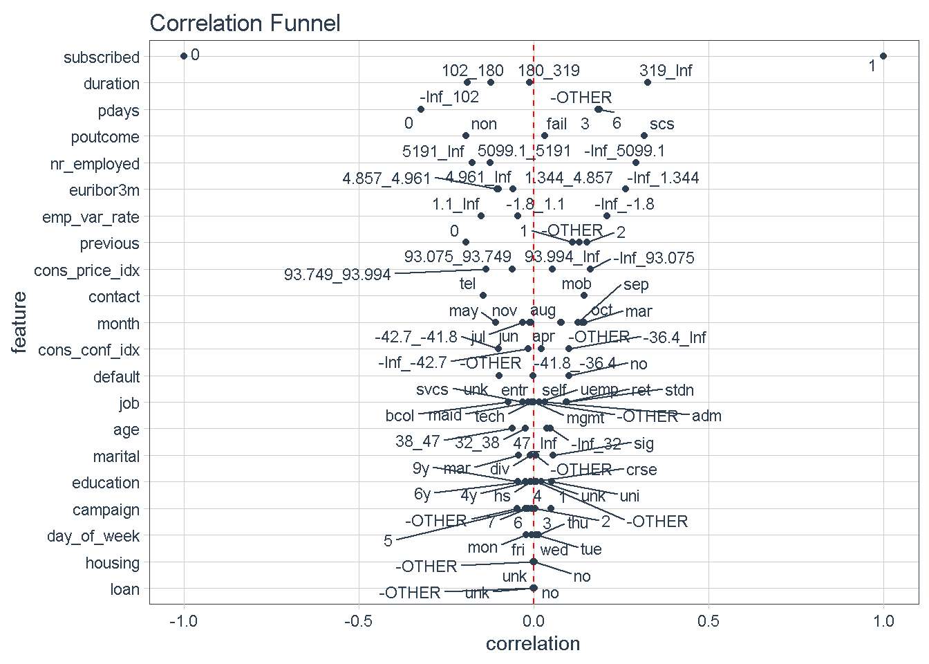
With 3 simple steps we can produce a graph that arranges predictors top to bottom in descending order of absolute correlation with the target variable. Features at the top of the funnel are expected to have have stronger predictive power in a model.
This approach offers a quick way to identify a hierarchy of expected predictive power for all variables and gives an early indication of which predictors should feature strongly/weakly in any model.
data_clean %>%
# turn numeric and categorical features into binary data
binarize(n_bins = 4, # bin number for converting features to discrete
thresh_infreq = 0.01 # thresh. for assign categ. features into "Other"
) %>%
# Correlate target variable to features in data set
correlate(target = subscribed__1) %>%
# correlation funnel visualisation
plot_correlation_funnel()
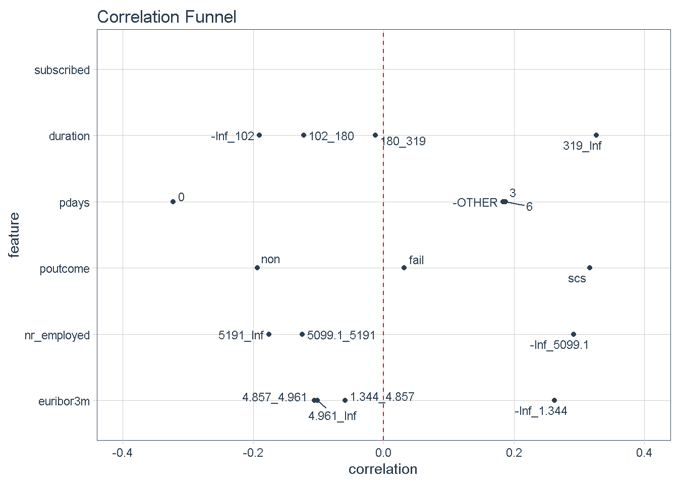
Zooming in on the top 5 features we can see that certain characteristics have a greater correlation with the target variable (subscribing to the term deposit product) when:
- The
durationof the last phone contact with the client is 319 seconds or longer - The number of
daysthat passed by after the client was last contacted is greater than 6 - The outcome of the
previousmarketing campaign wassuccess - The number of employed is 5,099 thousands or higher
- The value of the euribor 3 month rate is 1.344 or higher
.
data_clean %>%
select(subscribed, duration, pdays, poutcome, nr_employed, euribor3m) %>%
binarize(n_bins = 4, # bin number for converting numeric features to discrete
thresh_infreq = 0.01 # thresh. for assign categ. features into "Other"
) %>%
# Correlate target vriable to features in data set
correlate(target = subscribed__1) %>%
plot_correlation_funnel(limits = c(-0.4, 0.4))
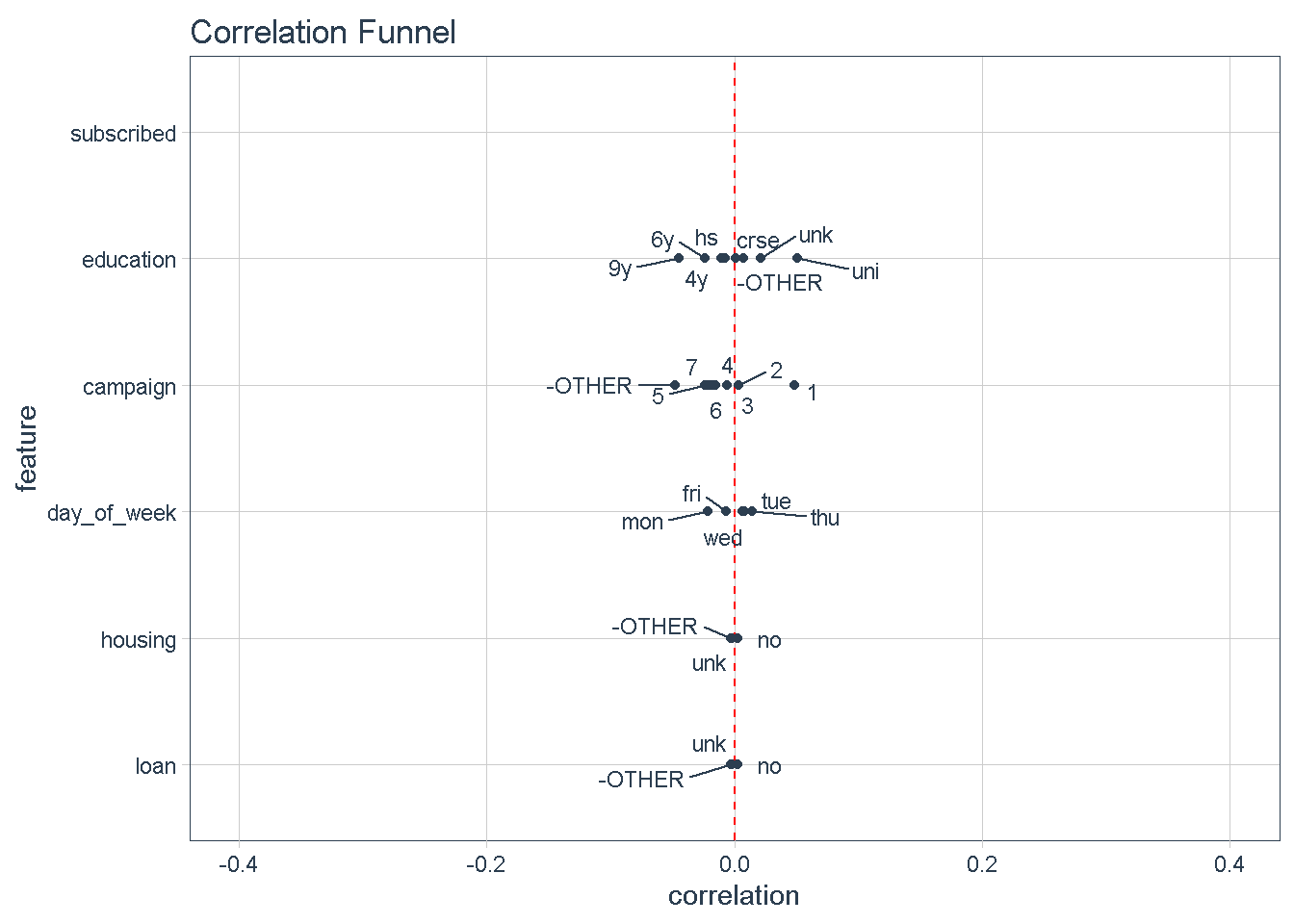
Conversely, variables at the bottom of the funnel, such as day_of_week, housing, and loan. show very little variation compared to the target variable (i.e.: they are very close to the zero correlation point to the response). For that reason, I’m not expecting these features to impact the response.
data_clean %>%
select(subscribed, education, campaign, day_of_week, housing, loan) %>%
binarize(n_bins = 4, # bin number for converting numeric features to discrete
thresh_infreq = 0.01 # thresh. for assign categ. features into "Other"
) %>%
# Correlate target vriable to features in data set
correlate(target = subscribed__1) %>%
plot_correlation_funnel(limits = c(-0.4, 0.4))
Features exploration
Guided by the results of this visual correlation analysis, I will continue to explore the relationship between the target and each of the predictors in the next section. For this I will enlist the help of the brilliant GGally library to visualise a modified version of the correlation matrix with Ggpairs, and plot mosaic charts with the ggmosaic package, a great way to examine the relationship among two or more categorical variables.
Target Variable
First things first, the target variable: subscribed shows a strong class imbalance, with nearly 89% in the No category to 11% in the Yes category.
data_clean %>%
select(subscribed) %>%
group_by(subscribed) %>%
count() %>%
# summarise(n = n()) %>% # alternative to count() - here you can name it!
ungroup() %>%
mutate(perc = n / sum(n)) %>%
ggplot(aes(x = subscribed, y = n, fill = subscribed) ) +
geom_col() +
geom_text(aes(label = scales::percent(perc, accuracy = 0.1)),
nudge_y = -2000,
size = 4.5) +
theme_minimal() +
theme(legend.position = 'none',
plot.title = element_text(hjust = 0.5)) +
labs(title = 'Target Variable',
x = 'Subscribed',
y = 'Number of Responses')
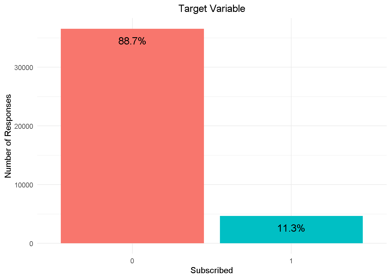
I am going to address class imbalance during the modelling phase by enabling re-sampling, in h2o. This will rebalance the dataset by “shrinking” the prevalent class (“No” or 0) and ensure that the model adequately detects what variables are driving the ‘yes’ and ‘no’ responses.
Predictors
Let’s continue with some of the numerical features:
data_clean %>%
select(subscribed, duration, age, pdays, previous) %>%
plot_ggpairs_funct(colour = subscribed)
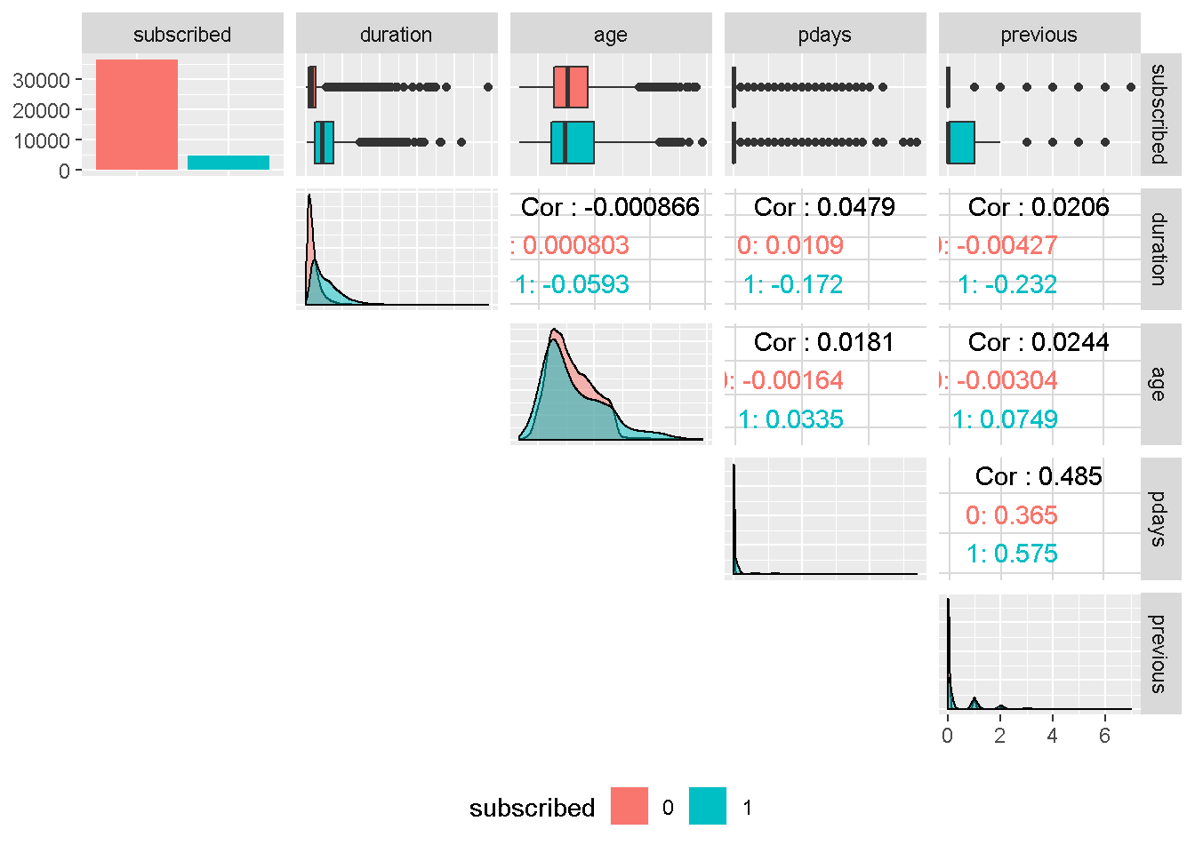
Although the correlation funnel analysis revealed that duration has the strongest expected predictive power, it is unknown before a call (it’s obviously known afterwards) and offers very little actionable insight or predictive value. Therefore, it should be discarded from any realistic predictive model and will not be used in this analysis.
age ’s density plots have very similar variance compared to the target variable and are centred around the same area. For these reasons, it should not have a great impact on subscribed.
Despite continuous in nature, pdays and previous are in fact categorical features and are also all strongly right skewed. For these reasons, they will need to be discretised into groups. Both variables are also moderately correlated, suggesting that they may capture the same behaviour.
Next, I visualise the bank client data with the mosaic charts:
job <- ggplot(data = data_clean) +
geom_mosaic(aes(x = product(job, subscribed), fill = job)) +
theme_minimal() +
theme(legend.position = 'none',
plot.title = element_text(hjust = 0.5) ) +
labs(x = '', y = '', title = 'Job')
mar <- ggplot(data = data_clean) +
geom_mosaic(aes(x = product(marital, subscribed), fill = marital)) +
theme_minimal() +
theme(legend.position = 'none',
plot.title = element_text(hjust = 0.5) ) +
labs(x = '', y = '', title = 'Marital')
edu <- ggplot(data = data_clean) +
geom_mosaic(aes(x = product(education, subscribed), fill = education)) +
theme_minimal() +
theme(legend.position = 'none',
plot.title = element_text(hjust = 0.5) ) +
labs(x = '', y = '', title = 'Education')
def <- ggplot(data = data_clean) +
geom_mosaic(aes(x = product(default, subscribed), fill = default)) +
theme_minimal() +
theme(legend.position = 'none',
plot.title = element_text(hjust = 0.5) ) +
labs(x = '', y = '', title = 'Default')
hou <- ggplot(data = data_clean) +
geom_mosaic(aes(x = product(housing, subscribed), fill = housing)) +
theme_minimal() +
theme(legend.position = 'none',
plot.title = element_text(hjust = 0.5) ) +
labs(x = '', y = '', title = 'Housing')
loa <- ggplot(data = data_clean) +
geom_mosaic(aes(x = product(loan, subscribed), fill = loan)) +
theme_minimal() +
theme(legend.position = 'none',
plot.title = element_text(hjust = 0.5) ) +
labs(x = '', y = '', title = 'Loan')
gridExtra::grid.arrange(job, mar, hou, edu, def, loa, nrow = 2)
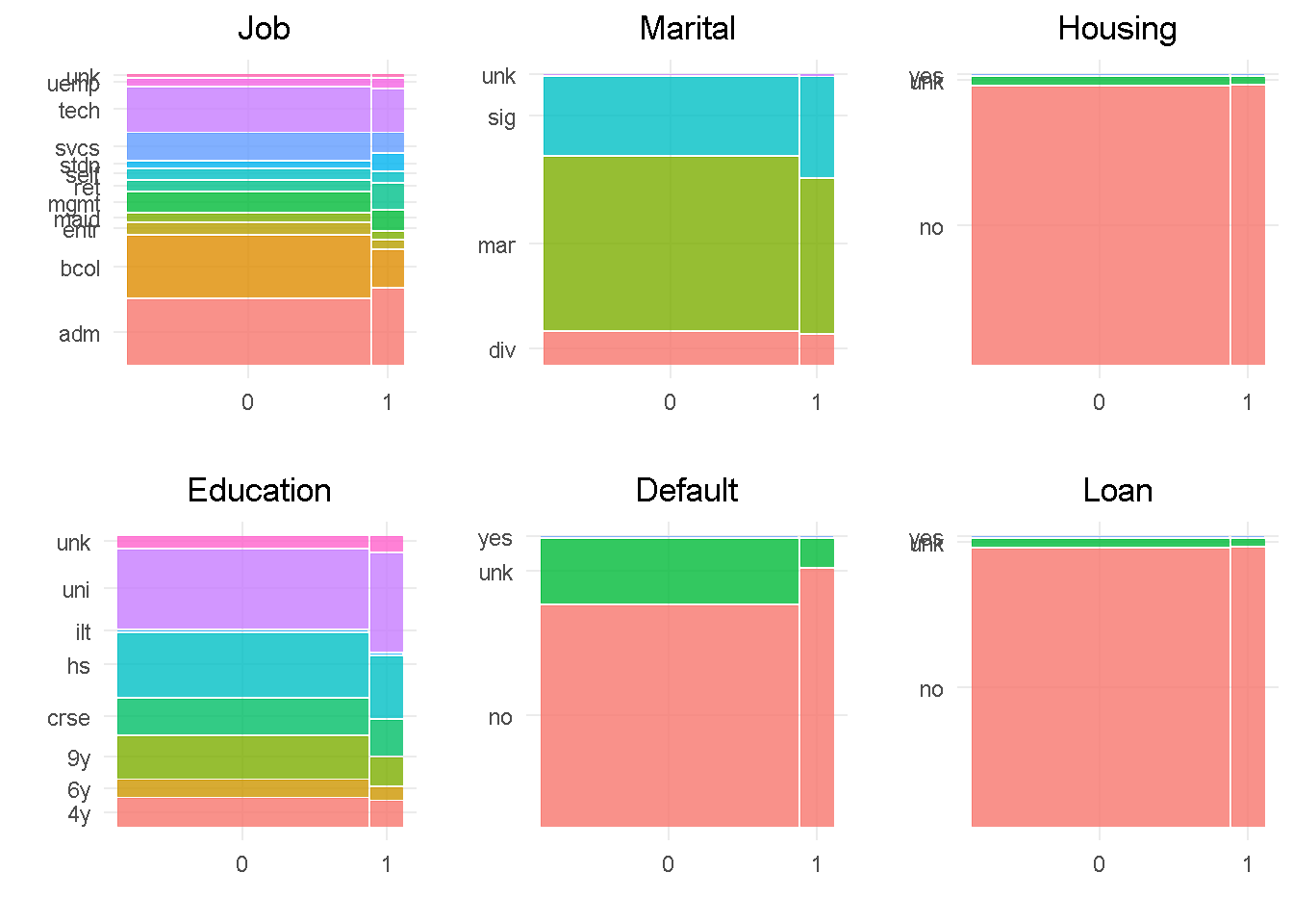
In line with the correlationfunnel findings, job, education, marital and default all show a good level of variation compared to the target variable, indicating that they would impact the response. In contrast, housing and loan sat at the very bottom of the funnel and are expected to have little influence on the target, given the small variation when split by “subscribed” response.
default has only 3 observations in the ‘yes’ level, which will be rolled into the least frequent level as they’re not enough to make a proper inference. Level ‘unknown’ of the housing and loan variables have a small number of observations and will be rolled into the second smallest category. Lastly, job and education would also benefit from grouping up of least common levels.
Moving on to the other campaign attributes:
data_clean %>%
select(subscribed, campaign, poutcome) %>%
plot_ggpairs_funct(colour = subscribed)

Although continuous in principal, campaign is more categorical in nature and strongly right skewed, and will need to be discretised into groups. However, we have learned from the earlier correlation analysis that is not expected be a strong drivers of variation in any model.
On the other hand, poutcome is one of the attributes expected to be have a strong predictive power. The uneven distribution of levels would suggest to roll the least common occurring level (success or scs) into another category. However, contacting a client who previously purchased a term deposit is one of the catacteristics with highest predictive power and needs to be left ungrouped.
Then, I’m looking at last contact information:
con <- ggplot(data = data_clean) +
geom_mosaic(aes(x = product(contact, subscribed), fill = contact)) +
theme_minimal() +
theme(legend.position = 'none',
plot.title = element_text(hjust = 0.5) ) +
labs(x = '', y = '', title = 'Contact')
mth <- ggplot(data = data_clean) +
geom_mosaic(aes(x = product(month, subscribed), fill = month)) +
theme_minimal() +
theme(legend.position = 'none',
plot.title = element_text(hjust = 0.5) ) +
labs(x = '', y = '', title = 'Month')
dow <- ggplot(data = data_clean) +
geom_mosaic(aes(x = product(day_of_week, subscribed), fill = day_of_week)) +
theme_minimal() +
theme(legend.position = 'none',
plot.title = element_text(hjust = 0.5) ) +
labs(x = '', y = '', title = 'Day of Week')
gridExtra::grid.arrange(con, mth, dow, nrow = 2)
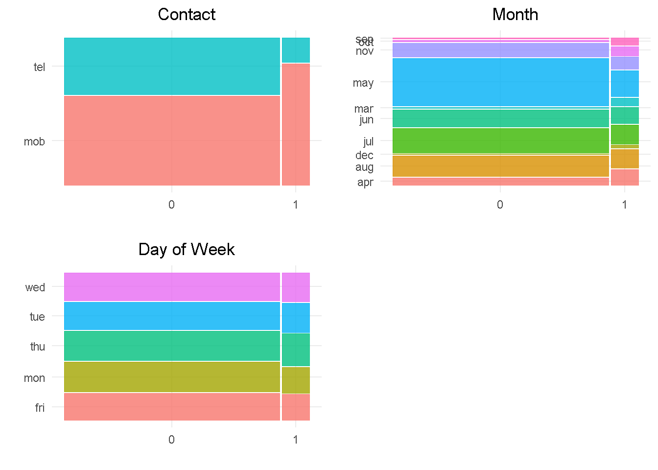
contact and month should impact the response variable as they both have a good level of variation compared to the target. month would also benefit from grouping up of least common levels.
In contrast, day_of_week does not appear to impact the response as there is not enough variation between the levels.
Last but not least, the social and economic attributes:
data_clean %>%
select(subscribed, emp_var_rate, cons_price_idx,
cons_conf_idx, euribor3m, nr_employed) %>%
plot_ggpairs_funct(colour = subscribed)
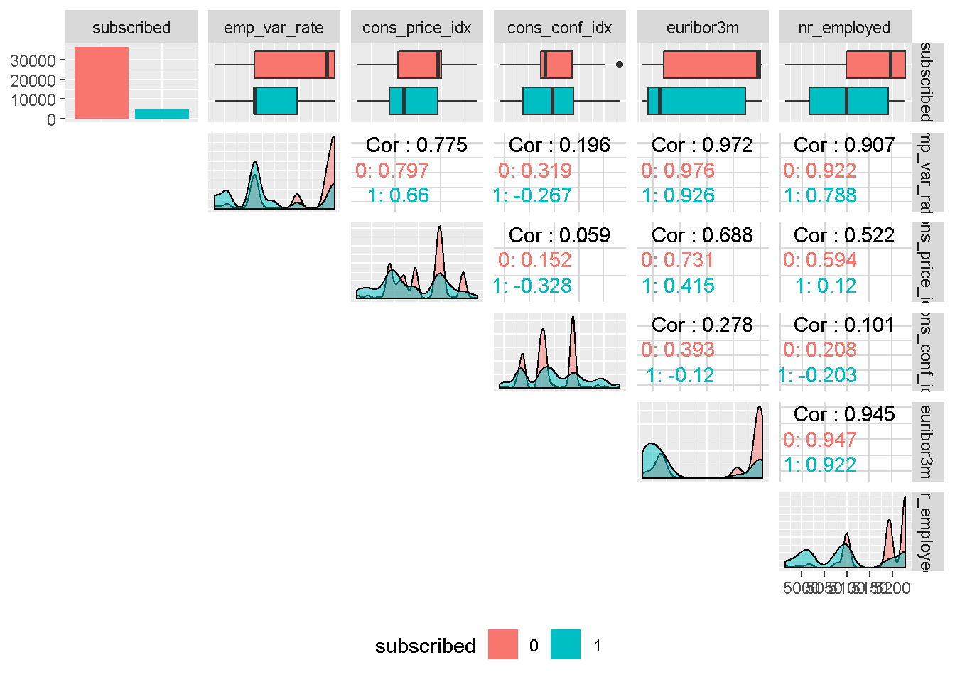
All social and economic attributes show a good level of variation compared to the target variable, which suggests that they should all impact the response. They all display a high degree of multi-modality and do not have an even spread through the density plot, and will need to be binned.
It is also worth noting that, with the exception of consumer confidence index, all other social and economic attributes are strongly correlated to each other, indicating that only one could be included in the model as they are all “picking up” similar economic trend.
Data Processing and Transformation
Following up on the findings from the Exploratory Data Analysis, I’m getting the data ready for modelling.
Discretising of categorical predictors
Here, I’m using a helper function plot_hist_funct to take a look at features histograms. That helps understanding how to combine least common levels into “other’ category.
data_clean %>%
select_if(is_character) %>%
plot_hist_funct()
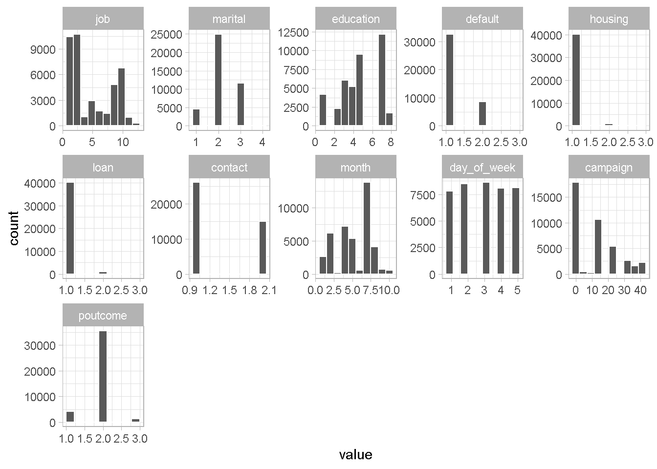
With the exception of day_of_week and contact, all categorical variables need some grouping up. I’m going to go through the first one as an example of how I approached the problem and include all changes made at the end.
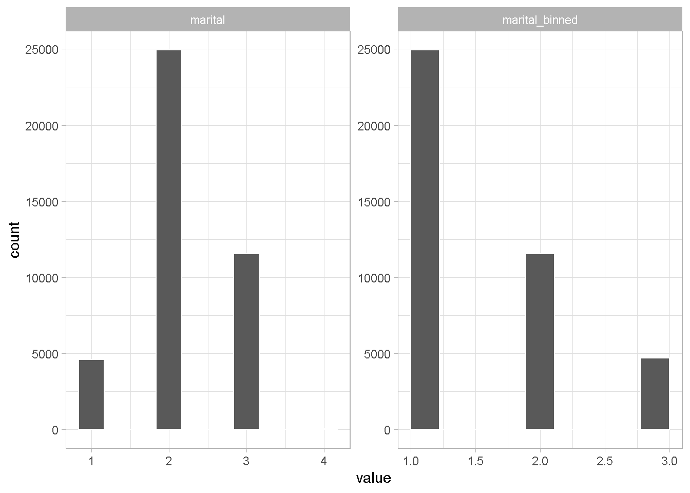
Example with marital status
A 3-bin combination seems sensible for the marital status category
data_clean %>%
# combine least common factors into "other' category
select(marital) %>%
mutate(marital_binned = marital %>% fct_lump(
# n = how many categs to keep
n = 2,
# name other category
other_level = "other"
)) %>%
plot_hist_funct()
Discretising of continuous variables
Using the same approach as to categorical variables, I’m plotting all numerical features.
data_clean %>%
select_if(is.numeric) %>%
plot_hist_funct()
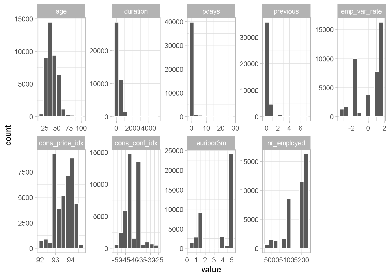
All continuous variables can benefit from some grouping. For simplicity and speed, I’m using the bins calculated by the correlationfunnel package. duration will not be processed as I’m NOT including it in any of my models.
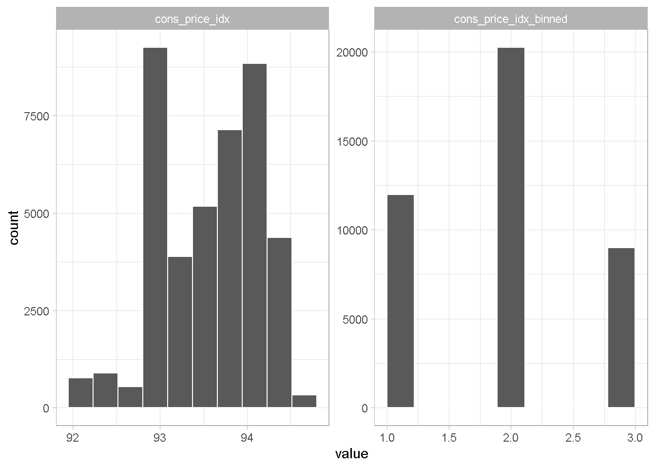
Example with consumer confidence index
A 3-level binning seems sensible for cons_price_idx
data_clean %>%
select(cons_price_idx) %>%
mutate(cons_price_idx_binned = case_when(
between(cons_price_idx, -Inf, 93.056) ~ "Inf_93.056",
between(cons_price_idx, 93.056, 93.912) ~ "93.056_93.912",
TRUE ~ "93.913_Inf")) %>%
plot_hist_funct()
I create now a data_final file with all the binned variables, set all categorical variables to factors and take a good look at all of them.
data_final <-
data_clean %>%
# removing duration, which I'm not going to use for modelling
select(-duration) %>%
# applying grouping
mutate(
job = job %>% fct_lump(n = 11, other_level = "other"),
marital = marital %>% fct_lump(n = 2, other_level = "other"),
education = education %>% fct_lump(n = 6, other_level = "other"),
default = default %>% fct_lump(n = 1, other_level = "other"),
housing = housing %>% fct_lump(n = 1, other_level = "other"),
loan = loan %>% fct_lump(n = 1, other_level = "other"),
# month = month %>% fct_lump(n = 6,other_level = "other"),
campaign = campaign %>% fct_lump(n = 3, other_level = "other"),
# poutcome = poutcome %>% fct_lump(n = 1, other_level = "other"),
pdays = case_when(
pdays == 0 ~ "Never",
TRUE ~ "Once_or_more"),
previous = case_when(
previous == 0 ~ "Never",
TRUE ~ "Once_or_more"),
emp_var_rate = case_when(
between(emp_var_rate, -Inf, -1.8) ~ "nInf_n1.8",
between(emp_var_rate, -1.9, -0.1) ~ "n1.9_n0.1",
TRUE ~ "n0.2_Inf"),
cons_price_idx = case_when(
between(cons_price_idx, -Inf, 93.056) ~ "nInf_93.056",
between(cons_price_idx, 93.057, 93.912) ~ "93.057_93.912",
TRUE ~ "93.913_Inf"),
cons_conf_idx = case_when(
between(cons_conf_idx, -Inf, -46.19) ~ "nInf_n46.19",
between(cons_conf_idx, -46.2, -41.99) ~ "n46.2_n41.9",
between(cons_conf_idx, -42.0, -39.99) ~ "n42.0_n39.9",
between(cons_conf_idx, -40.0, -36.39) ~ "n40.0_n36.4",
TRUE ~ "n36.5_Inf"),
euribor3m = case_when(
between(euribor3m, -Inf, 1.298) ~ "nInf_1.298",
between(euribor3m, 1.299, 4.190) ~ "1.299_4.190",
between(euribor3m, 1.191, 4.864) ~ "1.299_4.864",
between(euribor3m, 1.865, 4.862) ~ "1.299_4.962",
TRUE ~ "4.963_Inf"),
nr_employed = case_when(
between(nr_employed, -Inf, 5099.1) ~ "nInf_5099.1",
between(nr_employed, 5099.1, 5191.01) ~ "5099.1_5191.01",
TRUE ~ "5191.02_Inf")
) %>%
# change categorical variables to factors
mutate_at(c('contact', 'month', 'day_of_week', 'pdays', 'poutcome',
'previous', 'emp_var_rate', 'cons_price_idx',
'cons_conf_idx', 'euribor3m', 'nr_employed'),
as.factor)
It all looks fine!
data_final %>% str()
## Classes 'tbl_df', 'tbl' and 'data.frame': 41188 obs. of 20 variables:
## $ subscribed : Factor w/ 2 levels "0","1": 1 1 1 1 1 1 1 1 1 1 ...
## $ age : num 56 57 37 40 56 45 59 41 24 25 ...
## $ job : Factor w/ 12 levels "adm","bcol","entr",..: 4 9 9 1 9 9 1 2 10 9 ...
## $ marital : Factor w/ 3 levels "mar","sig","other": 1 1 1 1 1 1 1 1 2 2 ...
## $ education : Factor w/ 7 levels "4y","6y","9y",..: 1 5 5 2 5 3 4 7 4 5 ...
## $ default : Factor w/ 2 levels "no","other": 1 2 1 1 1 2 1 2 1 1 ...
## $ housing : Factor w/ 2 levels "no","other": 1 1 1 1 1 1 1 1 1 1 ...
## $ loan : Factor w/ 2 levels "no","other": 1 1 1 1 1 1 1 1 1 1 ...
## $ contact : Factor w/ 2 levels "mob","tel": 2 2 2 2 2 2 2 2 2 2 ...
## $ month : Factor w/ 10 levels "apr","aug","dec",..: 7 7 7 7 7 7 7 7 7 7 ...
## $ day_of_week : Factor w/ 5 levels "fri","mon","thu",..: 2 2 2 2 2 2 2 2 2 2 ...
## $ campaign : Factor w/ 4 levels "1","2","3","other": 1 1 1 1 1 1 1 1 1 1 ...
## $ pdays : Factor w/ 2 levels "Never","Once_or_more": 1 1 1 1 1 1 1 1 1 1 ...
## $ previous : Factor w/ 2 levels "Never","Once_or_more": 1 1 1 1 1 1 1 1 1 1 ...
## $ poutcome : Factor w/ 3 levels "fail","non","scs": 2 2 2 2 2 2 2 2 2 2 ...
## $ emp_var_rate : Factor w/ 3 levels "n0.2_Inf","n1.9_n0.1",..: 1 1 1 1 1 1 1 1 1 1 ...
## $ cons_price_idx: Factor w/ 3 levels "93.057_93.912",..: 2 2 2 2 2 2 2 2 2 2 ...
## $ cons_conf_idx : Factor w/ 5 levels "n36.5_Inf","n40.0_n36.4",..: 2 2 2 2 2 2 2 2 2 2 ...
## $ euribor3m : Factor w/ 4 levels "1.299_4.190",..: 2 2 2 2 2 2 2 2 2 2 ...
## $ nr_employed : Factor w/ 3 levels "5099.1_5191.01",..: 1 1 1 1 1 1 1 1 1 1 ...
Summary of Exploratory Data Analysis & Preparation
Correlation analysis with correlationfunnel helped identify a hierarchy of expected predictive power for all variables
duration has strongest correlation with target variable whereas some of the bank client data like housing and loan shows the weakest correlation
However, duration will NOT be used in the analysis as it is unknown before a call. As such it offers very little actionable insight or predictive value and should be discarded from any realistic predictive model
The target variable subscribed shows strong class imbalance, with nearly 89% of No churn, which will need to be addresses before the modelling analysis can begin
Most predictors benefited from grouping up of least common levels
Further feature exploration revealed the most social and economic context attributes are strongly correlated to each other, suggesting that only a selection of them could be considered in a final model
Save final dataset
Lastly, I save the data_final set for the next phase of the analysis.
# Saving clensed data for analysis phase
saveRDS(data_final, "../01_data/data_final.rds")
Code Repository
The full R code and all relevant data files can be found on my GitHub profile @ Propensity Modelling
References
For the original paper that used the data set see: A Data-Driven Approach to Predict the Success of Bank Telemarketing. Decision Support Systems, S. Moro, P. Cortez and P. Rita.
To Speed Up Exploratory Data Analysis see: correlationfunnel Package Vignette
Appendix
Table 1 – Variables Description
| Category | Attribute | Description | Type |
|---|---|---|---|
| Target | subscribed | has the client subscribed a term deposit? | binary: “yes”,“no” |
| Client Data | age | - | numeric |
| Client Data | job | type of job | categorical |
| Client Data | marital | marital status | categorical |
| Client Data | education | - | categorical |
| Client Data | default | has credit in default? | categorical: “no”,“yes”,“unknown” |
| Client Data | housing | has housing loan? | categorical: “no”,“yes”,“unknown” |
| Client Data | loan | has personal loan? | categorical:“no”,“yes”,“unknown” |
| Last Contact Info | contact | contact communication type | categorical:“cellular”,“telephone” |
| Last Contact Info | month | last contact month of year | categorical |
| Last Contact Info | day_of_week | last contact day of the week | categorical: “mon”,“tue”,“wed”,“thu”,“fri” |
| Last Contact Info | duration | last contact duration, in seconds | numeric |
| Campaigns attrib. | campaign | number of contacts during this campaign and for this client | numeric |
| Campaigns attrib. | pdays | number of days after client was last contacted from previous campaign | numeric; 999 means client was not previously contacted |
| Campaigns attrib. | previous | number of contacts before this campaign and for this client | numeric |
| Campaigns attrib. | poutcome | outcome of previous marketing campaign | categorical: “failure”,“nonexistent”,“success” |
| Social & Economic | emp.var.rate | employment variation rate - quarterly indicator | numeric |
| Social & Economic | cons.price.idx | consumer price index - monthly indicator | numeric |
| Social & Economic | cons.conf.idx | consumer confidence index - monthly indicator | numeric |
| Social & Economic | euribor3m | euribor 3 month rate - daily indicator | numeric |
| Social & Economic | nr.employed | number of employees - quarterly indicator | numeric |