Modelling with Tidymodels and Parsnip - A Tidy Approach to a Classification Problem
Recently I have completed the online course Business Analysis With R focused on applied data and business science with R, which introduced me to a couple of new modelling concepts and approaches. One that especially captured my attention is parsnip and its attempt to implement a unified modelling and analysis interface (similar to python’s scikit-learn) to seamlessly access several modelling platforms in R.
parsnip is the brainchild of RStudio’s Max Khun (of caret fame) and Davis Vaughan and forms part of tidymodels, a growing ensemble of tools to explore and iterate modelling tasks that shares a common philosophy (and a few libraries) with the tidyverse.
Although there are a number of packages at different stages in their development, I have decided to take tidymodels “for a spin”, so to speak, and create and execute a “tidy” modelling workflow to tackle a classification problem. My aim is to show how easy it is to fit a simple logistic regression in R’s glm and quickly switch to a cross-validated random forest using the ranger engine by changing only a few lines of code.
For this post in particular I’m focusing on four different libraries from the tidymodels suite: rsample for data sampling and cross-validation, recipes for data preprocessing, parsnip for model set up and estimation, and yardstick for model assessment.
Note that the focus is on modelling workflow and libraries interaction. For that reason, I am keeping data exploration and feature engineering to a minimum.
Set up
First, I load the packages I need for this analysis.
library(tidymodels)
library(skimr)
library(tibble)
For this project I am using the Telco Customer Churn from IBM Watson Analytics, one of IBM Analytics Communities. The data contains 7,043 rows, each representing a customer, and 21 columns for the potential predictors, providing information to forecast customer behaviour and help develop focused customer retention programmes.
Churn is the Dependent Variable and shows the customers who left within the last month. The dataset also includes details on the Services that each customer has signed up for, along with Customer Account and Demographic information.
telco <- readr::read_csv("WA_Fn-UseC_-Telco-Customer-Churn.csv")
telco %>%
skimr::skim()
## Skim summary statistics
## n obs: 7043
## n variables: 21
##
## -- Variable type:character --------------------------------------------------------------------------
## variable missing complete n min max empty n_unique
## Churn 0 7043 7043 2 3 0 2
## Contract 0 7043 7043 8 14 0 3
## customerID 0 7043 7043 10 10 0 7043
## Dependents 0 7043 7043 2 3 0 2
## DeviceProtection 0 7043 7043 2 19 0 3
## gender 0 7043 7043 4 6 0 2
## InternetService 0 7043 7043 2 11 0 3
## MultipleLines 0 7043 7043 2 16 0 3
## OnlineBackup 0 7043 7043 2 19 0 3
## OnlineSecurity 0 7043 7043 2 19 0 3
## PaperlessBilling 0 7043 7043 2 3 0 2
## Partner 0 7043 7043 2 3 0 2
## PaymentMethod 0 7043 7043 12 25 0 4
## PhoneService 0 7043 7043 2 3 0 2
## StreamingMovies 0 7043 7043 2 19 0 3
## StreamingTV 0 7043 7043 2 19 0 3
## TechSupport 0 7043 7043 2 19 0 3
##
## -- Variable type:numeric ----------------------------------------------------------------------------
## variable missing complete n mean sd p0 p25 p50
## MonthlyCharges 0 7043 7043 64.76 30.09 18.25 35.5 70.35
## SeniorCitizen 0 7043 7043 0.16 0.37 0 0 0
## tenure 0 7043 7043 32.37 24.56 0 9 29
## TotalCharges 11 7032 7043 2283.3 2266.77 18.8 401.45 1397.47
## p75 p100
## 89.85 118.75
## 0 1
## 55 72
## 3794.74 8684.8
There are a couple of things to notice here:
customerID is a unique identifier for each row. As such it has no descriptive or predictive power and it needs to be removed.
Given the relative small number of missing values in TotalCharges (only 11 of them) I am dropping them from the dataset.
telco <- telco %>% select(-customerID) %>% drop_na()
Modelling with tidymodels
To show the basic steps in the tidymodels framework I am fitting and evaluating a simple logistic regression model.
Train and test split
rsample provides a streamlined way to create a randomised training and test split of the original data.
set.seed(seed = 1972)
train_test_split <-
rsample::initial_split(
data = telco,
prop = 0.80
)
train_test_split
## <5626/1406/7032>
Of the 7,043 total customers, 5,626 have been assigned to the training set and 1,406 to the test set. I save them as train_tbl and test_tbl.
train_tbl <- train_test_split %>% training()
test_tbl <- train_test_split %>% testing()
A simple recipe
The recipes package uses a cooking metaphor to handle all the data preprocessing, like missing values imputation, removing predictors, centring and scaling, one-hot-encoding, and more.
First, I create a recipe where I define the transformations I want to apply to my data. In this case I create a simple recipe to change all character variables to factors.
Then, I “prep the recipe” by mixing the ingredients with prep. Here I have included the prep bit in the recipe function for brevity.
recipe_simple <- function(dataset) {
recipe(Churn ~ ., data = dataset) %>%
step_string2factor(all_nominal(), -all_outcomes()) %>%
prep(data = dataset)
}
Note that in order to avoid data leakage (e.g: transferring information from the train set into the test set), data should be “prepped” using the train_tbl only.
recipe_prepped <- recipe_simple(dataset = train_tbl)
Finally, to continue with the cooking metaphor, I “bake the recipe” to apply all preprocessing to the data sets.
train_baked <- bake(recipe_prepped, new_data = train_tbl)
test_baked <- bake(recipe_prepped, new_data = test_tbl)
Fit the model
parsnip is a relatively recent addition to the tidymodels suite and is probably the one I like best. This package offers a unified API that allows access to several machine learning packages without the need to learn the syntax of each individual one.
With 3 simple steps you can:
set the type of model you want to fit (here is a
logistic regression) and its mode (classification)decide which computational engine to use (
glmin this case)spell out the exact model specification to fit (I’m using all variables here) and what data to use (the baked train dataset)
logistic_glm <- logistic_reg(mode = "classification") %>% set_engine("glm") %>% fit(Churn ~ ., data = train_baked)
If you want to use another engine you can simply switch the set_engine argument (for logistic regression you can choose from glm, glmnet, stan, spark, and keras) and parsnip will take care of changing everything else for you behind the scenes.
Performance assessment
The yardstick package provides an easy way to calculate several assessment measures. But before I can evaluate my model’s performance, I need to calculate some predictions by passing the test_baked data to the predict function.
predictions_glm <- logistic_glm %>%
predict(new_data = test_baked) %>%
bind_cols(test_baked %>% select(Churn))
head(predictions_glm)
## # A tibble: 6 x 2
## .pred_class Churn
## <fct> <fct>
## 1 Yes No
## 2 No No
## 3 No No
## 4 No No
## 5 No No
## 6 No No
There are several metrics that can be used to investigate the performance of a classification model but for simplicity I’m only focusing on a selection of them: accuracy, precision, recall and F1_Score.
All of these measures (and many more) can be derived by the Confusion Matrix, a table used to describe the performance of a classification model on a set of test data for which the true values are known.
In and of itself, the confusion matrix is a relatively easy concept to get your head around as is shows the number of false positives, false negatives, true positives, and true negatives. However some of the measures that are derived from it may take some reasoning with to fully understand their meaning and use.
predictions_glm %>%
conf_mat(Churn, .pred_class) %>%
pluck(1) %>%
as_tibble() %>%
ggplot(aes(Prediction, Truth, alpha = n)) +
geom_tile(show.legend = FALSE) +
geom_text(aes(label = n), colour = "white", alpha = 1, size = 8)
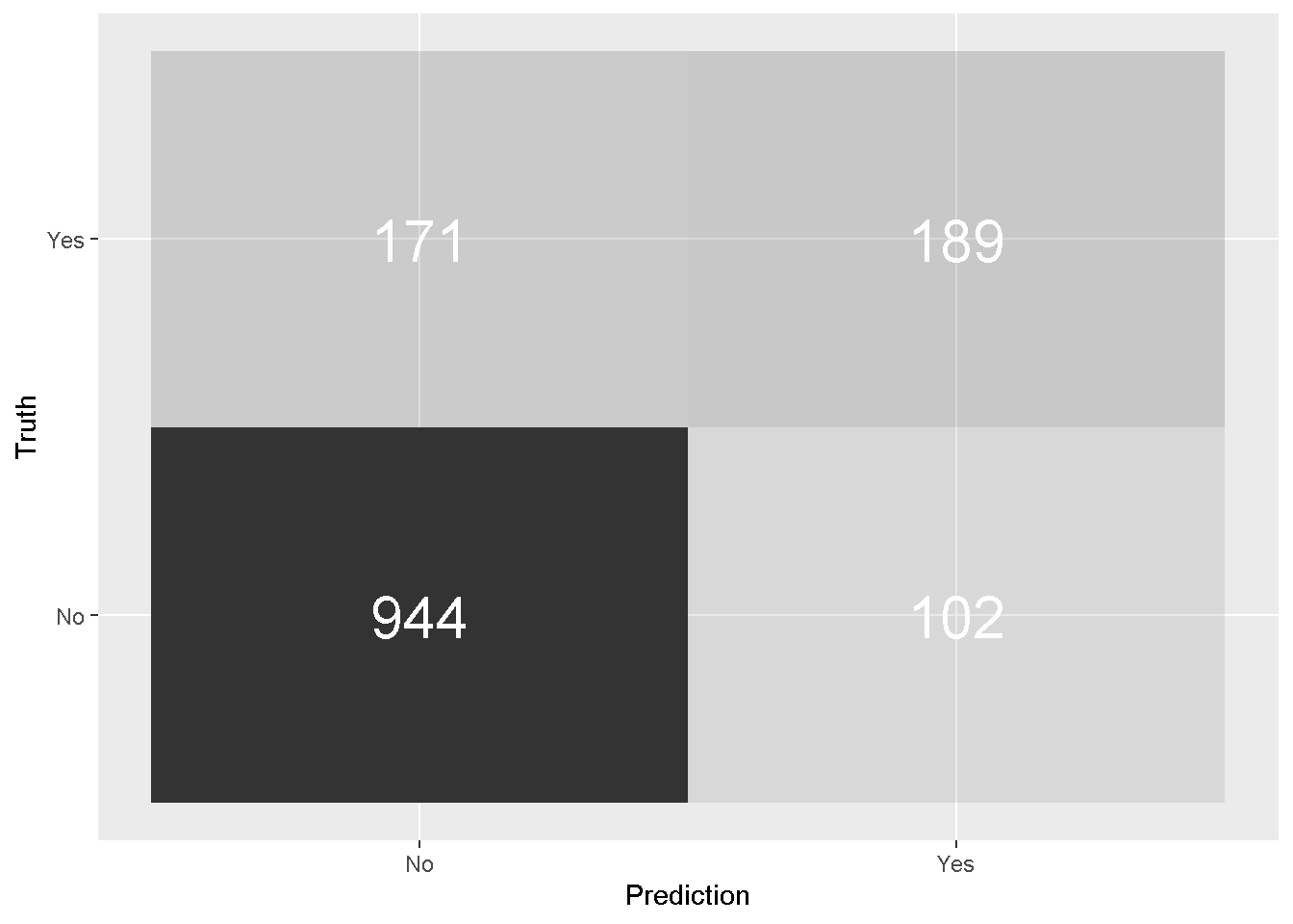
The model’s Accuracy is the fraction of predictions the model got right and can be easily calculated by passing the predictions_glm to the metrics function. However, accuracy is not a very reliable metric as it will provide misleading results if the data set is unbalanced.
With only basic data manipulation and feature engineering the simple logistic model has achieved 80% accuracy.
predictions_glm %>%
metrics(Churn, .pred_class) %>%
select(-.estimator) %>%
filter(.metric == "accuracy") %>%
kable()
| .metric | .estimate |
|---|---|
| accuracy | 0.8058321 |
Precision shows how sensitive models are to False Positives (i.e. predicting a customer is leaving when he-she is actually staying) whereas Recall looks at how sensitive models are to False Negatives (i.e. forecasting that a customer is staying whilst he-she is in fact leaving).
These are very relevant business metrics because organisations are particularly interested in accurately predicting which customers are truly at risk of leaving so that they can target them with retention strategies. At the same time they want to minimising efforts of retaining customers incorrectly classified as leaving who are instead staying.
tibble(
"precision" =
precision(predictions_glm, Churn, .pred_class) %>%
select(.estimate),
"recall" =
recall(predictions_glm, Churn, .pred_class) %>%
select(.estimate)
) %>%
unnest() %>%
kable()
| precision | recall |
|---|---|
| 0.8466368 | 0.9024857 |
Another popular performance assessment metric is the F1 Score, which is the harmonic average of the precision and recall. An F1 score reaches its best value at 1 with perfect precision and recall.
predictions_glm %>%
f_meas(Churn, .pred_class) %>%
select(-.estimator) %>%
kable()
| .metric | .estimate |
|---|---|
| f_meas | 0.8736696 |
A Random Forest
This is where the real beauty of tidymodels comes into play. Now I can use this tidy modelling framework to fit a Random Forest model with the ranger engine.
Cross-validation set up
To further refine the model’s predictive power, I am implementing a 10-fold cross validation using vfold_cv from rsample, which splits again the initial training data.
cross_val_tbl <- vfold_cv(train_tbl, v = 10)
cross_val_tbl
## # 10-fold cross-validation
## # A tibble: 10 x 2
## splits id
## <named list> <chr>
## 1 <split [5.1K/563]> Fold01
## 2 <split [5.1K/563]> Fold02
## 3 <split [5.1K/563]> Fold03
## 4 <split [5.1K/563]> Fold04
## 5 <split [5.1K/563]> Fold05
## 6 <split [5.1K/563]> Fold06
## 7 <split [5.1K/562]> Fold07
## 8 <split [5.1K/562]> Fold08
## 9 <split [5.1K/562]> Fold09
## 10 <split [5.1K/562]> Fold10
If we take a further look, we should recognise the 5,626 number, which is the total number of observations in the initial train_tbl. In each round, 563 observations will in turn be retained from estimation and used to validate the model for that fold.
cross_val_tbl$splits %>%
pluck(1)
## <5063/563/5626>
To avoid confusion and distinguish the initial train/test splits from those used for cross validation, the author of rsample Max Kuhn has coined two new terms: the analysis and the assessment sets. The former is the portion of the train data used to recursively estimate the model, where the latter is the portion used to validate each estimate.
Update the recipe
NOTE that a random forest needs all numeric variables to be centred and scaled and all character/factor variables to be “dummified”. This is easily done by updating the recipe with these transformations.
recipe_rf <- function(dataset) {
recipe(Churn ~ ., data = dataset) %>%
step_string2factor(all_nominal(), -all_outcomes()) %>%
step_dummy(all_nominal(), -all_outcomes()) %>%
step_center(all_numeric()) %>%
step_scale(all_numeric()) %>%
prep(data = dataset)
}
Estimate the model
Switching to another model could not be simpler! All I need to do is to change the type of model to random_forest and add its hyper-parameters, change the set_engine argument to ranger and I’m ready to go.
I’m bundling all steps into a function that estimates the model across all folds, runs predictions and returns a convenient tibble with all the results. I need to add an extra step before the recipe “prepping” to maps the cross validation splits to the analysis and assessment functions. This will guide the iterations through the 10 folds.
rf_fun <- function(split, id, try, tree) {
analysis_set <- split %>% analysis()
analysis_prepped <- analysis_set %>% recipe_rf()
analysis_baked <- analysis_prepped %>% bake(new_data = analysis_set)
model_rf <-
rand_forest(
mode = "classification",
mtry = try,
trees = tree
) %>%
set_engine("ranger",
importance = "impurity"
) %>%
fit(Churn ~ ., data = analysis_baked)
assessment_set <- split %>% assessment()
assessment_prepped <- assessment_set %>% recipe_rf()
assessment_baked <- assessment_prepped %>% bake(new_data = assessment_set)
tibble(
"id" = id,
"truth" = assessment_baked$Churn,
"prediction" = model_rf %>%
predict(new_data = assessment_baked) %>%
unlist()
)
}
Performance assessment
All I have left to do is mapping the formula to a data frame.
pred_rf <- map2_df(
.x = cross_val_tbl$splits,
.y = cross_val_tbl$id,
~ rf_fun(split = .x, id = .y, try = 3, tree = 200)
)
head(pred_rf)
## # A tibble: 6 x 3
## id truth prediction
## <chr> <fct> <fct>
## 1 Fold01 Yes Yes
## 2 Fold01 Yes No
## 3 Fold01 Yes Yes
## 4 Fold01 No No
## 5 Fold01 No No
## 6 Fold01 Yes No
I’ve found that yardstick has a very handy confusion matrix summary function, which returns an array of 13 different metrics but in this case I want to see the four I used for the glm model.
pred_rf %>%
conf_mat(truth, prediction) %>%
summary() %>%
select(-.estimator) %>%
filter(.metric %in%
c("accuracy", "precision", "recall", "f_meas")) %>%
kable()
| .metric | .estimate |
|---|---|
| accuracy | 0.7979026 |
| precision | 0.8250436 |
| recall | 0.9186301 |
| f_meas | 0.8693254 |
The random forest model is performing in par with the simple logistic regression. Given the very basic feature engineering that I’ve carried out, there is scope to further improve the model but this is beyond the scope of this post.
Closing considerations
One of the great advantage of tidymodels is the flexibility and ease of access to every phase of the analysis workflow. Creating the modelling pipeline is a breeze and you can easily re-use the initial framework by changing model type with parsnip and data pre-processing with recipes and in no time you’re ready to check your new model’s performance with yardstick.
In any analysis you would typically audit several models and parsnip frees you up from having to learn the unique syntax of every modelling engine so that you can focus on finding the best solution for the problem at hand.
Code repository
The full R code can be found on my GitHub profile
References
- Big thanks to Bruno Rodrigues for the article that provided the inspiration for the big evaluation formula A tutorial on tidy cross-validation with R
- More thanks to Benjamin Sorensen for his thoughtful piece on Modeling with
parsnipandtidymodels - For an introduction to
parsnip