Market Basket Analysis - Part 1 of 3 - Data Preparation and Exploratory Data Analysis
My objective for this piece of work is to carry out a Market Basket Analysis as an end-to-end data science project. I have split the output into three parts, of which this is the FIRST, that I have organised as follows:
In the first chapter, I will source, explore and format a complex dataset suitable for modelling with recommendation algorithms.
For the second part, I will apply various machine learning algorithms for Product Recommendation and select the best performing model. This will be done with the support of the recommenderlab package.
In the third and final instalment, I will implement the selected model in a Shiny Web Application.
Introduction
Market Basket Analysis or MBA (also referred to as Affinity Analysis) is a set of data mining and data analysis techniques used to understand customers shopping behaviours and uncover relationships among the products that they buy. By analysing the likes of retail basket composition, transactional data, or browsing history, these methods can be used to suggest to customers items they might be interested in. Such recommendations can promote customer loyalty, increase conversion rate by helping customers to find relevant products faster and boost cross-selling and up-selling by suggesting additional items or services.
Recommendation systems are widely employed in several industries. Online retailer Amazon uses these methods to recommend to their customers products that other people often buy together (‘customers who bought this item also bought…’). Every Monday since 2015 entertainment company Spotify suggests to their users a tailored playlist of 30 songs they’ve never listened to based on their consumption history. In 2009 Netflix famously ran a competition (The Netflix Prize) which awarded a $1M Grand Prize to the team that improved the predictions of their movie recommendation system.
Market Basket Analysis also finds applications in such areas as:
Promotions: MBA may give indications on how to structure promotion calendars. When two items (say, torch & batteries) are often bought together, a retailer may decide to have only one item on promotion to boost sales of the other.
Store Design: store layout can be shaped to place closer together items which are more often bought at the same time (e.g. milk & cereals, shampoo & conditioner, meat & vegetables, etc.)
Loyalty Programmes: when a customer has been inactive for some time, he/she can be prompted to re-engage with customised offers based on their purchase history.
Types of recommendation systems
There are several types of recommendation systems, each with their advantages and drawbacks.
I’ve arranged below a brief overview of some of the most known and used methods - please click on the tabs to have a look.
Association Rules
Association Rules analyses items most frequently purchased together to discover strong patterns in the data. Rules associating any pair of purchased items are establish using three metrics: “Support”, “Confidence”, and “Lift”:
Supportis the probability of two items being purchased together. P(Item1 & Item2)Confidenceis Support divided by the probability of buying Item2. Support / P(Item2)Liftis Confidence divided by the probability of buying Item1. Confidence / P(Item1)
The item with the highest Lift is the one most likely to be purchased. One drawback is that this approach doesn’t take into consideration the user’s purchase history.
Popular Items
As the name suggests, recommendations are based on general purchasing trends. Suggestions come from a list of most frequently purchased items that the customer has not yet bought. The main limitation for this approach is that the advice may not be entirely relevant to the customer.
Content-based Filtering
A content-based recommendation system investigates a client’s purchase history to understand hers/his preferences and recommends items similar to those the client has liked in the past. However, this approach relies on detailed transaction information, which may not always be available.
Collaborative Filtering
When a collaborative filtering is used, the recommendation system looks at either clients purchase history or clients product rating history. These are compiled into a user-item ratings matrix, with items (e.g. products) in the columns and users (e.g. customers or orders) in the rows. A measure of similarity is then calculated using methods like Cosine, Pearsons or Jaccard similarity to identify a hierarchy of probability to purchase.
Two methodologies are made use of:
User-based collaborative filtering (UBCF) focuses on similarities between users market basket composition to find other users with similar baskets. Similarity measures are then calculated and used to shape the suggestions list.
Item-based collaboartive filtering (IBCF) employes a similar appsoach but focuses instead on similarities between items that are frequently purchased together.
Hybrid Systems
Hybrid systems try to combine some of the approaches to overcome their limitations. There is a rich literature available online, in particular on the combining of collaborative filtering and content-based filtering, which in some cases have shown to be more effective than the pure approaches.
The Wikipedia article on Hybrid recommender systems also makes a very good read on the subject.
Data
The data for this project comes from the UCI Machine Learning Repository, an online archive of large datasets which includes a wide variety of data types, analysis tasks, and application areas.
In this project I’m using the Online Retail dataset, donated to UCI in 2015 by the School of Engineering at London South Bank University. This is a transnational dataset containing transactions occurring between 01/Dec/2010 and 09/Dec/2011 for a UK-based and registered online retail company. The company sells mainly unique all-occasion gifts and many of their customers are wholesalers.
For clarity and completeness, I’m including here the variables description
| Attribute | Description |
|---|---|
| InvoiceNo | Invoice number. 6-digit integral number. Indicates cancellation if starts with ‘C’ |
| StockCode | Product (item) code. 5-digit integral number |
| Description | Product (item) name |
| Quantity | The quantities of each product (item) per transaction. Numeric |
| InvoiceDate | Invoice Date and Time when each transaction was generated |
| UnitPrice | Unit price. Numeric, Product price per unit in sterling |
| CustomerID | Customer number. 5-digit integral number unique to each customer |
| Country | Country name. The name of the country where each customer resides |
I’ve picked this particular dataset because of it’s “real life” nature, which shows in the many manually entered annotations and adjustment codes I found in the Description field. There are even personal comments left by the company’s employees, who likely used the database on a day-to-day basis.
It’s reasonable to assume that the dataset came straight from the company’s database with very little alterations. From experience this is consistent with the state in which an analyst is most likely to receive data from a clients they are to conduct a piece of analysis for.
Data Preparation
Loading the Packages
# Importing libraries
library(data.table)
library(readxl)
library(tidyverse)
library(lubridate)
library(skimr)
library(knitr)
library(treemap)
Loading and Inspecting the Data
# import raw data file and trim leading and trailing whitespaces
retail <- read_excel("Online Retail.xlsx", trim_ws = TRUE)
The dataset consists of just over 540,000 observations spread across 8 variables. A few Descriptions and several CustomerIDs are missing and there are also some odd negatives Quantity and UnitPrice that would be worth investigating. It’s also worth noting that InvoiceDate is of POSIXct format, from which information about Date and Time of purchase can be extracted.
# First glance at the data
retail %>% skim()
## Skim summary statistics
## n obs: 541909
## n variables: 8
##
## -- Variable type:character --------------------------------------------------------------------------
## variable missing complete n min max empty n_unique
## Country 0 541909 541909 3 20 0 38
## Description 1454 540455 541909 1 35 0 4211
## InvoiceNo 0 541909 541909 6 7 0 25900
## StockCode 0 541909 541909 1 12 0 4070
##
## -- Variable type:numeric ----------------------------------------------------------------------------
## variable missing complete n mean sd p0 p25
## CustomerID 135080 406829 541909 15287.69 1713.6 12346 13953
## Quantity 0 541909 541909 9.55 218.08 -80995 1
## UnitPrice 0 541909 541909 4.61 96.76 -11062.06 1.25
## p50 p75 p100
## 15152 16791 18287
## 3 10 80995
## 2.08 4.13 38970
##
## -- Variable type:POSIXct ----------------------------------------------------------------------------
## variable missing complete n min max median
## InvoiceDate 0 541909 541909 2010-12-01 2011-12-09 2011-07-19
## n_unique
## 23260
Cancellations
The very handy Variables Description, which I’ve included above, tells us that if the InvoiceNo starts with letter ‘C’, it indicates a cancellation
retail %>%
filter(grepl("C", retail$InvoiceNo)) %>%
summarise(Total = n())
## # A tibble: 1 x 1
## Total
## <int>
## 1 9288
Cancellations are not needed for the analysis so they can be removed
retail <- retail %>%
filter(!grepl("C", retail$InvoiceNo))
# CHECK: total row count - 532,621
Negative Quantities
When filtering by non positive Quantity, the Description shows what looks like a series of manually entered comments (e.g.“thrown away”, “Unsaleable”, “damaged”,“?”). Given that UnitPrice is also set to zero for all of them, it is safe to assume that these were adjustments codes.
retail %>%
filter(Quantity <= 0) %>%
group_by(Description, UnitPrice) %>%
summarise(count = n()) %>%
arrange(desc(count)) %>%
ungroup()
## # A tibble: 139 x 3
## Description UnitPrice count
## <chr> <dbl> <int>
## 1 <NA> 0 862
## 2 check 0 120
## 3 damages 0 45
## 4 damaged 0 42
## 5 ? 0 41
## 6 sold as set on dotcom 0 20
## 7 Damaged 0 14
## 8 thrown away 0 9
## 9 Unsaleable, destroyed. 0 9
## 10 ?? 0 7
## # ... with 129 more rows
Were this a live project, I would typically sense check this assumption with whomever provided the data. In this case, I will simply remove all rows with non-positive Quantity.
retail <- retail %>%
filter(Quantity > 0)
# CHECK: total row count - 531,285
Non-Product StockCodes
Turning my attention to StockCode, I notice a handful of non-product related codes (‘Postage’, ‘Bank Charges’, ‘Gift Vouchers’, etc.).
# Non-product related codes
stc <- c('AMAZONFEE', 'BANK CHARGES', 'C2', 'DCGSSBOY', 'DCGSSGIRL',
'DOT', 'gift_0001_', 'PADS', 'POST')
retail %>%
filter(grepl(paste(stc, collapse = "|"), StockCode)) %>%
group_by(StockCode, Description) %>%
summarise(count = n()) %>%
arrange(desc(count)) %>%
ungroup()
## # A tibble: 19 x 3
## StockCode Description count
## <chr> <chr> <int>
## 1 POST POSTAGE 1126
## 2 DOT DOTCOM POSTAGE 708
## 3 C2 CARRIAGE 141
## 4 DCGSSGIRL GIRLS PARTY BAG 13
## 5 BANK CHARGES Bank Charges 12
## 6 DCGSSBOY BOYS PARTY BAG 11
## 7 gift_0001_20 Dotcomgiftshop Gift Voucher £20.00 9
## 8 gift_0001_10 Dotcomgiftshop Gift Voucher £10.00 8
## 9 gift_0001_30 Dotcomgiftshop Gift Voucher £30.00 7
## 10 gift_0001_50 Dotcomgiftshop Gift Voucher £50.00 4
## 11 PADS PADS TO MATCH ALL CUSHIONS 4
## 12 POST <NA> 4
## 13 gift_0001_40 Dotcomgiftshop Gift Voucher £40.00 3
## 14 AMAZONFEE AMAZON FEE 2
## 15 C2 <NA> 1
## 16 DOT <NA> 1
## 17 gift_0001_10 <NA> 1
## 18 gift_0001_20 to push order througha s stock was 1
## 19 gift_0001_30 <NA> 1
These can all be removed.
retail <- filter(retail, !grepl(paste(stc, collapse = "|"), StockCode))
# CHECK: total row count - 529,228
Description
Focusing now on the Description field, there are an additional 50 manually entered annotations that need removing. I one case an employee has even vented out their frustration at one of their co-workers (“alan hodge cant mamage this section”), with misspelling and all!
# Additional adjustment codes to remove
descr <- c( "check", "check?", "?", "??", "damaged", "found",
"adjustment", "Amazon", "AMAZON", "amazon adjust",
"Amazon Adjustment", "amazon sales", "Found", "FOUND",
"found box", "Found by jackie ", "Found in w/hse", "dotcom",
"dotcom adjust", "allocate stock for dotcom orders ta", "FBA",
"Dotcomgiftshop Gift Voucher £100.00", "on cargo order",
"wrongly sold (22719) barcode", "wrongly marked 23343",
"dotcomstock", "rcvd be air temp fix for dotcom sit", "Manual",
"John Lewis", "had been put aside", "for online retail orders",
"taig adjust", "amazon", "incorrectly credited C550456 see 47",
"returned", "wrongly coded 20713", "came coded as 20713",
"add stock to allocate online orders", "Adjust bad debt",
"alan hodge cant mamage this section", "website fixed",
"did a credit and did not tick ret", "michel oops",
"incorrectly credited C550456 see 47", "mailout", "test",
"Sale error", "Lighthouse Trading zero invc incorr", "SAMPLES",
"Marked as 23343", "wrongly coded 23343","Adjustment",
"rcvd be air temp fix for dotcom sit", "Had been put aside."
)
Filtering out the unwanted entries.
retail <- retail %>%
filter(!Description %in% descr)
# CHECK: total row count - 528,732
Last but not least, there are also some 600 NAs in Description.
sum(is.na(retail$Description))
## [1] 584
Potentially, I could have used StockCode to derive the missing entries, but given their small number (around 0.1% of total) I’ve opted to just remove them.
retail <- retail %>%
filter(!is.na(Description))
# CHECK: total row count - 528,148
Customer ID
There is still a significant number of NAs in CustomerID, which I will leave as they are.
retail$CustomerID %>%
skim()
##
## Skim summary statistics
##
## -- Variable type:numeric ----------------------------------------------------------------------------
## variable missing complete n mean sd p0 p25 p50 p75
## . 131778 396370 528148 15301.6 1709.98 12346 13975 15159 16803
## p100
## 18287
As I will discuss in the modelling part, for the analysis I need to arrange data in a user-item format, where “users” can be either customers or orders. Given that there are almost 5 times as many Orders as there are Customers, I am going to use InvoiceNo for orders in the analysis, which should make for a richer information set.
sapply(retail[,c('InvoiceNo','CustomerID')], function(x) length(unique(x)))
## InvoiceNo CustomerID
## 19792 4336
Final touches
There are a couple of housekeeping tasks to sort out and I am ready to go!
retail <- retail %>%
# Setting 'Description' and 'Country' as factors
mutate(Description = as.factor(Description)) %>%
mutate(Country = as.factor(Country)) %>%
# Changing 'InvoiceNo' type to numeric
mutate(InvoiceNo = as.numeric(InvoiceNo)) %>%
# Extracting 'Date' and 'Time' from 'InvoiceDate'
mutate(Date = as.Date(InvoiceDate)) %>%
mutate(Time = as.factor(format(InvoiceDate,"%H:%M:%S")))
glimpse(retail)
## Observations: 528,148
## Variables: 10
## $ InvoiceNo <dbl> 536365, 536365, 536365, 536365, 536365, 536365, 53...
## $ StockCode <chr> "85123A", "71053", "84406B", "84029G", "84029E", "...
## $ Description <fct> WHITE HANGING HEART T-LIGHT HOLDER, WHITE METAL LA...
## $ Quantity <dbl> 6, 6, 8, 6, 6, 2, 6, 6, 6, 32, 6, 6, 8, 6, 6, 3, 2...
## $ InvoiceDate <dttm> 2010-12-01 08:26:00, 2010-12-01 08:26:00, 2010-12...
## $ UnitPrice <dbl> 2.55, 3.39, 2.75, 3.39, 3.39, 7.65, 4.25, 1.85, 1....
## $ CustomerID <dbl> 17850, 17850, 17850, 17850, 17850, 17850, 17850, 1...
## $ Country <fct> United Kingdom, United Kingdom, United Kingdom, Un...
## $ Date <date> 2010-12-01, 2010-12-01, 2010-12-01, 2010-12-01, 2...
## $ Time <fct> 08:26:00, 08:26:00, 08:26:00, 08:26:00, 08:26:00, ...
Exploratory Data Analysis
And I am now ready to start exploring the dataset different features.
What items do people buy more often?
The heart-shaped tea light holder is the most popular item.
retail %>%
group_by(Description) %>%
summarize(count = n()) %>%
top_n(10, wt = count) %>%
arrange(desc(count)) %>%
ggplot(aes(x = reorder(Description, count), y = count)) +
geom_bar(stat = "identity", fill = "royalblue", colour = "blue") +
labs(x = "", y = "Top 10 Best Sellers") +
coord_flip() +
theme_grey(base_size = 12)
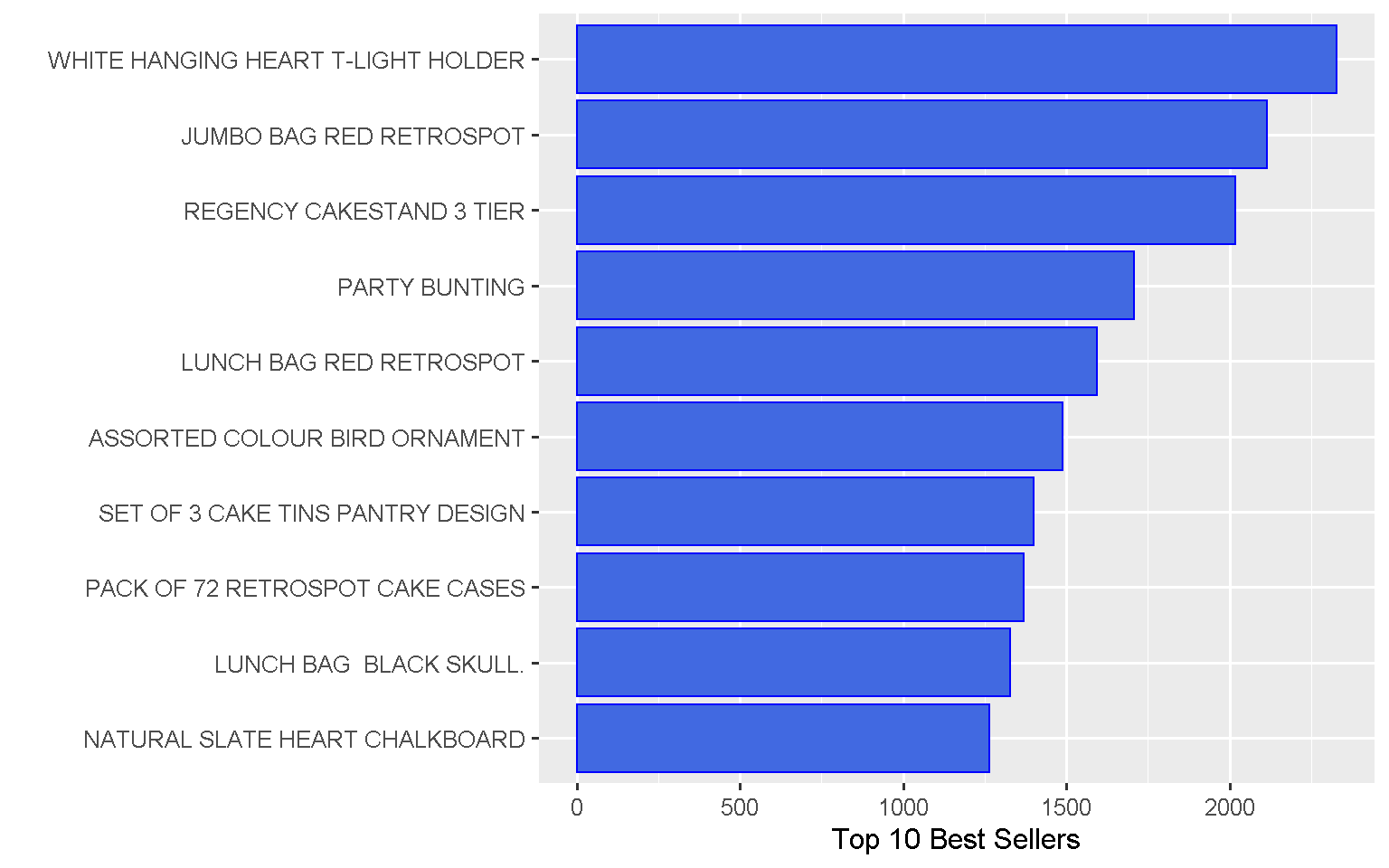
Top 10 most sold products represent around 3% of total items sold by the company
retail %>%
group_by(Description) %>%
summarize(count = n()) %>%
mutate(pct = (count/sum(count))*100) %>%
arrange(desc(pct)) %>%
ungroup() %>%
top_n(10, wt = pct)
## # A tibble: 10 x 3
## Description count pct
## <fct> <int> <dbl>
## 1 WHITE HANGING HEART T-LIGHT HOLDER 2327 0.441
## 2 JUMBO BAG RED RETROSPOT 2115 0.400
## 3 REGENCY CAKESTAND 3 TIER 2019 0.382
## 4 PARTY BUNTING 1707 0.323
## 5 LUNCH BAG RED RETROSPOT 1594 0.302
## 6 ASSORTED COLOUR BIRD ORNAMENT 1489 0.282
## 7 SET OF 3 CAKE TINS PANTRY DESIGN 1399 0.265
## 8 PACK OF 72 RETROSPOT CAKE CASES 1370 0.259
## 9 LUNCH BAG BLACK SKULL. 1328 0.251
## 10 NATURAL SLATE HEART CHALKBOARD 1263 0.239
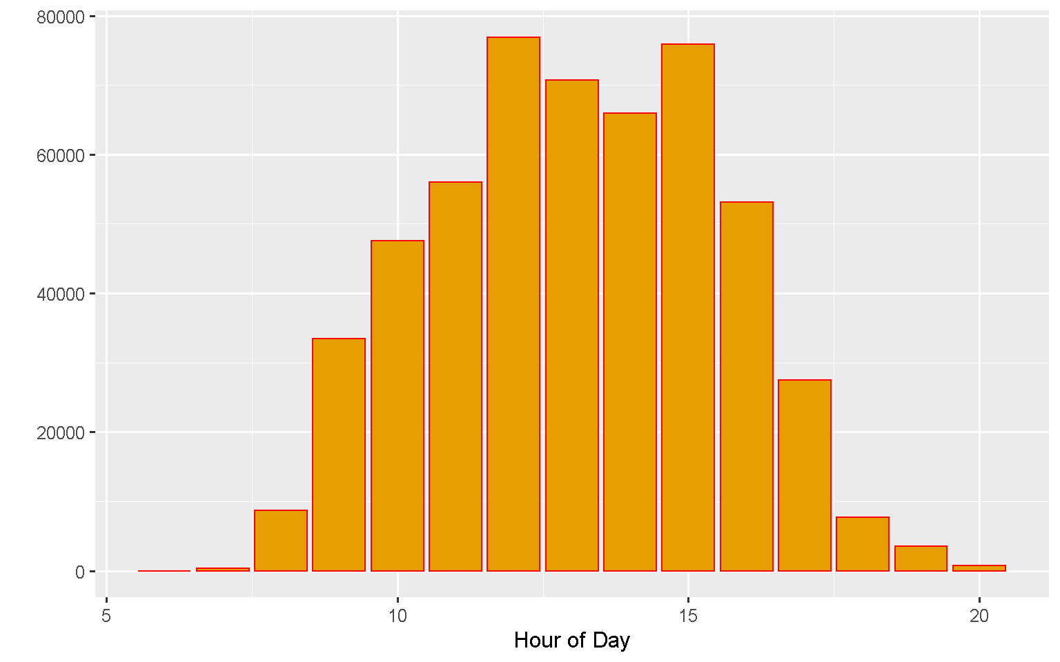
What time of day do people buy more often?
Lunchtime is the preferred time for shopping online, with the majority of orders places between 12 noon and 3pm.
retail %>%
ggplot(aes(hour(hms(Time)))) +
geom_histogram(stat = "count",fill = "#E69F00", colour = "red") +
labs(x = "Hour of Day", y = "") +
theme_grey(base_size = 12)
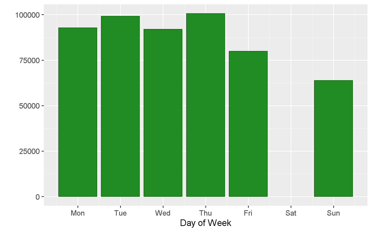
What day of the week do people buy more often?
Orders peaks on Thursdays with no orders processed on Saturdays.
retail %>%
ggplot(aes(wday(Date,
week_start = getOption("lubridate.week.start", 1)))) +
geom_histogram(stat = "count" , fill = "forest green", colour = "dark green") +
labs(x = "Day of Week", y = "") +
scale_x_continuous(breaks = c(1,2,3,4,5,6,7),
labels = c("Mon", "Tue", "Wed", "Thu", "Fri", "Sat", "Sun")) +
theme_grey(base_size = 14)
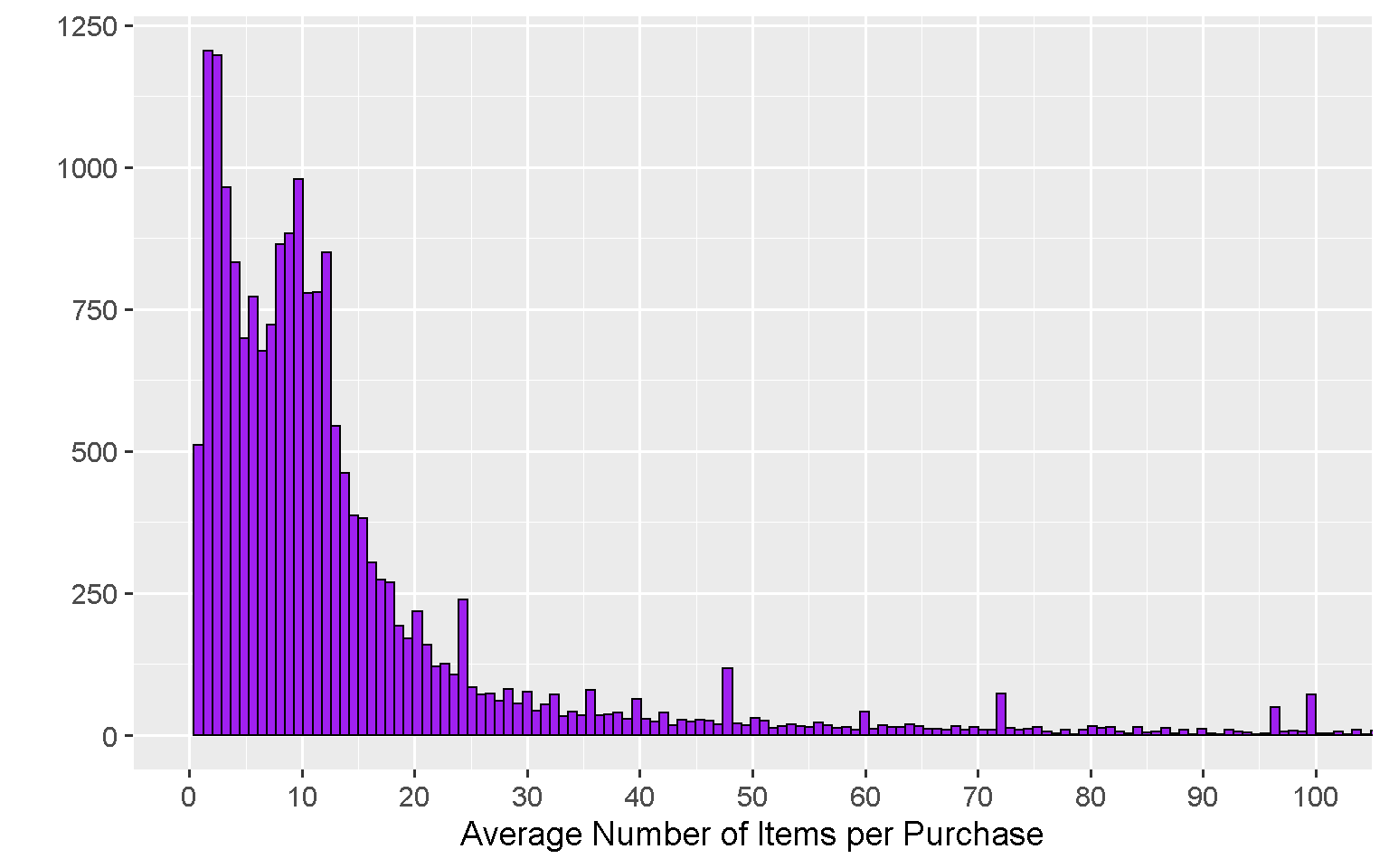
How many items does each customer buy?
The large majority of customers typically purchase between 2 and 15 items, with a peak at 2.
retail %>%
group_by(InvoiceNo) %>%
summarise(n = mean(Quantity)) %>%
ggplot(aes(x = n)) +
geom_histogram(bins = 100000, fill = "purple", colour = "black") +
coord_cartesian(xlim = c(0,100)) +
scale_x_continuous(breaks = seq(0,100,10)) +
labs(x = "Average Number of Items per Purchase", y = "") +
theme_grey(base_size = 14)
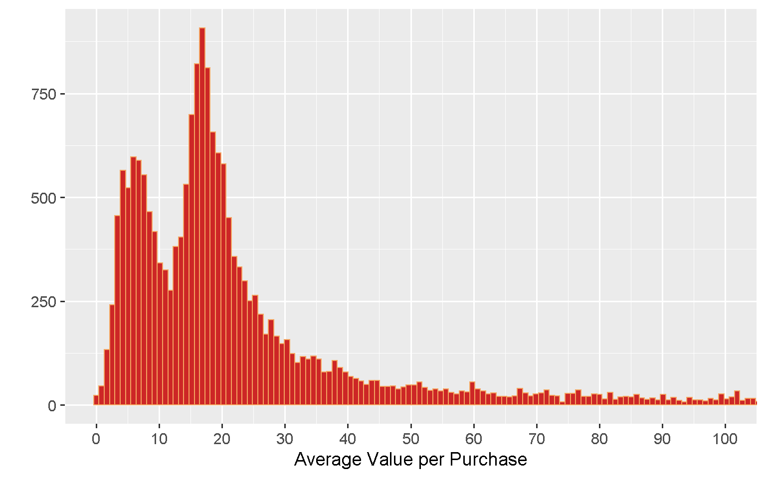
What is the average value per order?
The bulk of orders have a value below £20, with the distribution showing a double peak, one at £6 and a more pronounced one at £17.
retail %>%
mutate(Value = UnitPrice * Quantity) %>%
group_by(InvoiceNo) %>%
summarise(n = mean(Value)) %>%
ggplot(aes(x = n)) +
geom_histogram(bins = 200000, fill = "firebrick3", colour = "sandybrown") +
coord_cartesian(xlim = c(0,100)) +
scale_x_continuous(breaks = seq(0,100,10)) +
labs(x = "Average Value per Purchase", y = "") +
theme_grey(base_size = 14)
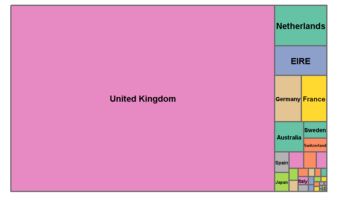
Which countries do they sell their goods to?
Five sixths of the orders come from the United Kingdom.
treemap(retail,
index = c("Country"),
vSize = "Quantity",
title = "",
palette = "Set2",
border.col = "grey40")
Comments
This concludes the data preparation and visualisation part of the project. I have removed Cancellations, eliminated negative Quantity and UnitPrice, got rid of NAs in Description and created two new variables, Date and Time. A total of 13,761 rows (roughly 2.5% of the initial count) were discarded and the dataset has now 528,148 observations.
Code Repository
The full R code can be found on my GitHub profile
References
- For Recommenderlab Package see: https://cran.r-project.org/package=recommenderlab
- For Recommenderlab Package Vignette see: https://cran.r-project.org/web/packages/recommenderlab/vignettes/recommenderlab.pdf