Market Basket Analysis - Part 2 of 3 - Market Basket Analysis with recommenderlab
My objective for this piece of work is to carry out a Market Basket Analysis as an end-to-end data science project. I have split the output into three parts, of which this is the SECOND, that I have organised as follows:
In the first chapter, I will source, explore and format a complex dataset suitable for modelling with recommendation algorithms.
For the second part, I will apply various machine learning algorithms for Product Recommendation and select the best performing model. This will be done with the support of the recommenderlab package.
In the third and final instalment, I will implement the selected model in a Shiny Web Application.
Loading the Packages
# Importing libraries
library(data.table)
library(tidyverse)
library(knitr)
library(recommenderlab)
The Data
For the analysis I will be using the retail dataset prepared and cleansed in Part 1.
glimpse(retail)
## Observations: 528,148
## Variables: 10
## $ InvoiceNo <dbl> 536365, 536365, 536365, 536365, 536365, 536365, 53...
## $ StockCode <chr> "85123A", "71053", "84406B", "84029G", "84029E", "...
## $ Description <fct> WHITE HANGING HEART T-LIGHT HOLDER, WHITE METAL LA...
## $ Quantity <dbl> 6, 6, 8, 6, 6, 2, 6, 6, 6, 32, 6, 6, 8, 6, 6, 3, 2...
## $ InvoiceDate <dttm> 2010-12-01 08:26:00, 2010-12-01 08:26:00, 2010-12...
## $ UnitPrice <dbl> 2.55, 3.39, 2.75, 3.39, 3.39, 7.65, 4.25, 1.85, 1....
## $ CustomerID <dbl> 17850, 17850, 17850, 17850, 17850, 17850, 17850, 1...
## $ Country <fct> United Kingdom, United Kingdom, United Kingdom, Un...
## $ Date <date> 2010-12-01, 2010-12-01, 2010-12-01, 2010-12-01, 2...
## $ Time <fct> 08:26:00, 08:26:00, 08:26:00, 08:26:00, 08:26:00, ...
Modelling
For the analysis part of this project I am using recommenderlab, an R package which provides a convenient framework to evaluate and compare various recommendation algorithms and quickly establish the best performing one.
Create the Rating Matrix
I now need to arrange the purchase history in a ratings matrix, with orders in rows and products in columns. This format is often called user-item matrix because “users” (e.g. customers or orders) tend to be on the rows and “items” (e.g. products) on the columns.
recommenderlab accepts 2 types of rating matrix for modelling:
real rating matrix consisting of actual user ratings, which requires normalisation.
binary rating matrix consisting of 0’s and 1’s, where 1’s indicate if the product was purchased. This is the matrix type needed for the analysis and it does not require normalisation.
However, when creating the rating matrix, it becomes apparent that some orders contain the same item more than once, as shown in the example below.
retail %>%
# Filtering by an order number which contains the same stock code more than once
filter(InvoiceNo == 557886 & StockCode == 22436) %>%
select(InvoiceNo, StockCode, Quantity, UnitPrice, CustomerID)
## # A tibble: 2 x 5
## InvoiceNo StockCode Quantity UnitPrice CustomerID
## <dbl> <chr> <dbl> <dbl> <dbl>
## 1 557886 22436 1 0.65 17799
## 2 557886 22436 3 0.65 17799
It is possible that the company that donated this dataset to the UCI Machine Learning Repository had an order processing system that allowed for an item to be added multiple times to the same order. For this analysis, I only need to know if an item was included in an order, so these duplicates need to be removed.
retail <- retail %>%
# create unique identifier
mutate(InNo_Desc = paste(InvoiceNo, Description, sep = ' '))
# filter out duplicates and drop unique identifier
retail <- retail[!duplicated(retail$InNo_Desc), ] %>%
select(-InNo_Desc)
# CHECK: total row count - 517,354
I can now create the rating matrix.
ratings_matrix <- retail %>%
# Select only needed variables
select(InvoiceNo, Description) %>%
# Add a column of 1s
mutate(value = 1) %>%
# Spread into user-item format
spread(Description, value, fill = 0) %>%
select(-InvoiceNo) %>%
# Convert to matrix
as.matrix() %>%
# Convert to recommenderlab class 'binaryRatingsMatrix'
as("binaryRatingMatrix")
ratings_matrix
## 19792 x 4001 rating matrix of class 'binaryRatingMatrix' with 517354 ratings.
Evaluation Scheme and Model Validation
In order to establish the models effectiveness, recommenderlab implements a number of evaluation schemes.
In this scheme, I split the data into a train set and a test set by selecting train = 0.8 for a 80⁄20 train/test split. I have also set method = “cross” and k = 5 for a 5-fold cross validation. This means that the data is divided into k subsets of equal size, with 80% of the data used for training and the remaining 20% used for evaluation. The models are recursively estimated 5 times, each time using a different train/test split, which ensures that all users and items are considered for both training and testing. The results can then be averaged to produce a single evaluation.
Selecting given = -1 means that for the test users ‘all but 1’ randomly selected item is withheld for evaluation.
scheme <- ratings_matrix %>%
evaluationScheme(method = "cross",
k = 5,
train = 0.8,
given = -1)
scheme
## Evaluation scheme using all-but-1 items
## Method: 'cross-validation' with 5 run(s).
## Good ratings: NA
## Data set: 19792 x 4001 rating matrix of class 'binaryRatingMatrix' with 517354 ratings.
Set up List of Algorithms
One of recommenderlab main features is the ability to estimate multiple algorithms in one go. First, I create a list with the algorithms I want to estimate, specifying all the models parameters. Here, I consider schemes which evaluate on a binary rating matrix and include the random items algorithm for benchmarking purposes.
algorithms <- list(
"association rules" = list(name = "AR", param = list(supp = 0.01, conf = 0.01)),
"random items" = list(name = "RANDOM", param = NULL),
"popular items" = list(name = "POPULAR", param = NULL),
"item-based CF" = list(name = "IBCF", param = list(k = 5)),
"user-based CF" = list(name = "UBCF", param = list(method = "Cosine", nn = 500))
)
Estimate the Models
All I have to do now is to pass scheme and algoritms to the evaluate() function, select type = topNList to evaluate a Top N List of product recommendations and specify how many recommendations to calculate with the parameter n = c(1, 3, 5, 10, 15, 20).
Please note that the CF based algorithms take a few minutes each to estimate.
results <- recommenderlab::evaluate(scheme,
algorithms,
type = "topNList",
n = c(1, 3, 5, 10, 15, 20)
)
## AR run fold/sample [model time/prediction time]
## 1 [0.27sec/60.24sec]
## 2 [0.25sec/58.55sec]
## 3 [0.23sec/58.34sec]
## 4 [0.24sec/57.89sec]
## 5 [0.22sec/58.05sec]
## RANDOM run fold/sample [model time/prediction time]
## 1 [0sec/18.83sec]
## 2 [0sec/18.46sec]
## 3 [0sec/17.96sec]
## 4 [0sec/18.33sec]
## 5 [0sec/18.42sec]
## POPULAR run fold/sample [model time/prediction time]
## 1 [0.02sec/22.34sec]
## 2 [0sec/22.29sec]
## 3 [0sec/22.51sec]
## 4 [0.01sec/22.24sec]
## 5 [0.01sec/22.6sec]
## IBCF run fold/sample [model time/prediction time]
## 1 [503.96sec/2.78sec]
## 2 [499.74sec/2.51sec]
## 3 [498.91sec/2.65sec]
## 4 [499.47sec/2.66sec]
## 5 [500.53sec/2.66sec]
## UBCF run fold/sample [model time/prediction time]
## 1 [0sec/287.46sec]
## 2 [0sec/286.23sec]
## 3 [0sec/286.87sec]
## 4 [0sec/286.46sec]
## 5 [0sec/287.82sec]
The output is stored as a list containing all the evaluations.
results
## List of evaluation results for 5 recommenders:
## Evaluation results for 5 folds/samples using method 'AR'.
## Evaluation results for 5 folds/samples using method 'RANDOM'.
## Evaluation results for 5 folds/samples using method 'POPULAR'.
## Evaluation results for 5 folds/samples using method 'IBCF'.
## Evaluation results for 5 folds/samples using method 'UBCF'.
Results for each single model can be easily retrieved and inspected.
results$'popular' %>%
getConfusionMatrix()
## [[1]]
## TP FP FN TN precision recall
## 1 0.005808081 0.9941919 0.9941919 4000.006 0.005808081 0.005808081
## 3 0.022727273 2.9772727 0.9772727 3998.023 0.007575758 0.022727273
## 5 0.031818182 4.9681818 0.9681818 3996.032 0.006363636 0.031818182
## 10 0.048232323 9.9517677 0.9517677 3991.048 0.004823232 0.048232323
## 15 0.061363636 14.9386364 0.9386364 3986.061 0.004090909 0.061363636
## 20 0.075505051 19.9244949 0.9244949 3981.076 0.003775253 0.075505051
## TPR FPR
## 1 0.005808081 0.0002484859
## 3 0.022727273 0.0007441321
## 5 0.031818182 0.0012417350
## 10 0.048232323 0.0024873201
## 15 0.061363636 0.0037337257
## 20 0.075505051 0.0049798788
##
## [[2]]
## TP FP FN TN precision recall
## 1 0.007575758 0.9924242 0.9924242 4000.008 0.007575758 0.007575758
## 3 0.026262626 2.9737374 0.9737374 3998.026 0.008754209 0.026262626
## 5 0.036111111 4.9638889 0.9638889 3996.036 0.007222222 0.036111111
## 10 0.054797980 9.9452020 0.9452020 3991.055 0.005479798 0.054797980
## 15 0.067171717 14.9328283 0.9328283 3986.067 0.004478114 0.067171717
## 20 0.081313131 19.9186869 0.9186869 3981.081 0.004065657 0.081313131
## TPR FPR
## 1 0.007575758 0.0002480440
## 3 0.026262626 0.0007432485
## 5 0.036111111 0.0012406621
## 10 0.054797980 0.0024856791
## 15 0.067171717 0.0037322740
## 20 0.081313131 0.0049784271
##
## [[3]]
## TP FP FN TN precision recall
## 1 0.007828283 0.9921717 0.9921717 4000.008 0.007828283 0.007828283
## 3 0.023989899 2.9760101 0.9760101 3998.024 0.007996633 0.023989899
## 5 0.031818182 4.9681818 0.9681818 3996.032 0.006363636 0.031818182
## 10 0.048989899 9.9510101 0.9510101 3991.049 0.004898990 0.048989899
## 15 0.063888889 14.9361111 0.9361111 3986.064 0.004259259 0.063888889
## 20 0.076010101 19.9239899 0.9239899 3981.076 0.003800505 0.076010101
## TPR FPR
## 1 0.007828283 0.0002479809
## 3 0.023989899 0.0007438166
## 5 0.031818182 0.0012417350
## 10 0.048989899 0.0024871307
## 15 0.063888889 0.0037330945
## 20 0.076010101 0.0049797525
##
## [[4]]
## TP FP FN TN precision recall
## 1 0.01035354 0.9896465 0.9896465 4000.010 0.010353535 0.01035354
## 3 0.02676768 2.9732323 0.9732323 3998.027 0.008922559 0.02676768
## 5 0.03737374 4.9626263 0.9626263 3996.037 0.007474747 0.03737374
## 10 0.05328283 9.9467172 0.9467172 3991.053 0.005328283 0.05328283
## 15 0.06590909 14.9340909 0.9340909 3986.066 0.004393939 0.06590909
## 20 0.08055556 19.9194444 0.9194444 3981.081 0.004027778 0.08055556
## TPR FPR
## 1 0.01035354 0.0002473498
## 3 0.02676768 0.0007431223
## 5 0.03737374 0.0012403465
## 10 0.05328283 0.0024860578
## 15 0.06590909 0.0037325896
## 20 0.08055556 0.0049786165
##
## [[5]]
## TP FP FN TN precision recall
## 1 0.008080808 0.9919192 0.9919192 4000.008 0.008080808 0.008080808
## 3 0.019949495 2.9800505 0.9800505 3998.020 0.006649832 0.019949495
## 5 0.029545455 4.9704545 0.9704545 3996.030 0.005909091 0.029545455
## 10 0.047727273 9.9522727 0.9522727 3991.048 0.004772727 0.047727273
## 15 0.060858586 14.9391414 0.9391414 3986.061 0.004057239 0.060858586
## 20 0.072727273 19.9272727 0.9272727 3981.073 0.003636364 0.072727273
## TPR FPR
## 1 0.008080808 0.0002479178
## 3 0.019949495 0.0007448264
## 5 0.029545455 0.0012423031
## 10 0.047727273 0.0024874463
## 15 0.060858586 0.0037338519
## 20 0.072727273 0.0049805730
Visualise results
recommenderlab has a basic plot function that can be used to compare models performance. However, I prefer to sort out the results in a tidy format for added flexibility and charting customisation.
First, I arrange the confusion matrix output for one model in a convenient format.
# Pull into a list all confusion matrix information for one model
tmp <- results$`user-based CF` %>%
getConfusionMatrix() %>%
as.list()
# Calculate average value of 5 cross-validation rounds
as.data.frame( Reduce("+",tmp) / length(tmp)) %>%
# Add a column to mark the number of recommendations calculated
mutate(n = c(1, 3, 5, 10, 15, 20)) %>%
# Select only columns needed and sorting out order
select('n', 'precision', 'recall', 'TPR', 'FPR')
## n precision recall TPR FPR
## 1 1 0.07657364 0.07656566 0.07656566 0.0002307756
## 2 3 0.04621678 0.13863636 0.13863636 0.0007150864
## 3 5 0.03507422 0.17535354 0.17535354 0.0012057339
## 4 10 0.02335587 0.23353535 0.23353535 0.0024407534
## 5 15 0.01837223 0.27555556 0.27555556 0.0036798124
## 6 20 0.01533237 0.30661616 0.30661616 0.0049216105
Then, I put the previous steps into a formula.
avg_conf_matr <- function(results) {
tmp <- results %>%
getConfusionMatrix() %>%
as.list()
as.data.frame( Reduce("+",tmp) / length(tmp)) %>%
mutate(n = c(1, 3, 5, 10, 15, 20)) %>%
select('n', 'precision', 'recall', 'TPR', 'FPR')
}
Next, I use the map() function from the purrr package to get all results in a tidy format, ready for charting.
# Using map() to iterate function across all models
results_tbl <- results %>%
map(avg_conf_matr) %>%
# Turning into an unnested tibble
enframe() %>%
# Unnesting to have all variables on same level
unnest()
results_tbl
## # A tibble: 30 x 6
## name n precision recall TPR FPR
## <chr> <dbl> <dbl> <dbl> <dbl> <dbl>
## 1 association rules 1 0.0432 0.0355 0.0355 0.000196
## 2 association rules 3 0.0324 0.0722 0.0722 0.000578
## 3 association rules 5 0.0282 0.0977 0.0977 0.000943
## 4 association rules 10 0.0230 0.135 0.135 0.00178
## 5 association rules 15 0.0207 0.158 0.158 0.00254
## 6 association rules 20 0.0191 0.171 0.171 0.00324
## 7 random items 1 0.000152 0.000152 0.000152 0.000250
## 8 random items 3 0.000202 0.000606 0.000606 0.000750
## 9 random items 5 0.000273 0.00136 0.00136 0.00125
## 10 random items 10 0.000232 0.00232 0.00232 0.00250
## # ... with 20 more rows
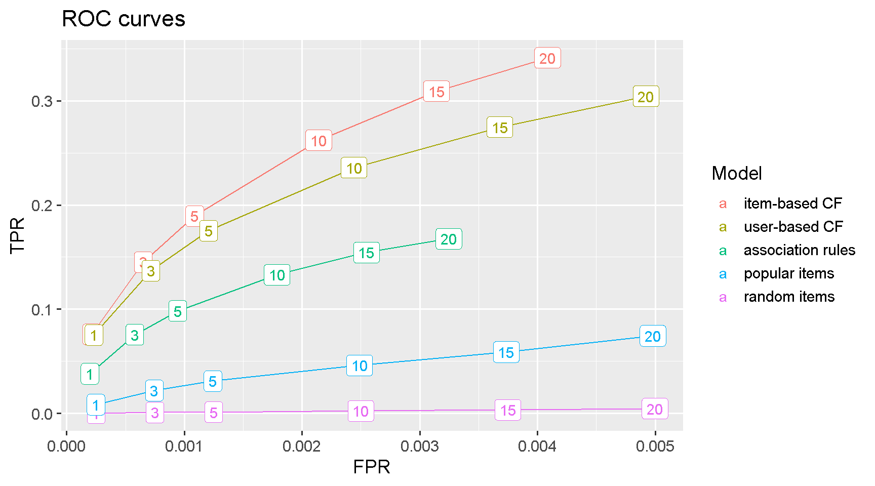
ROC curve
Classification models performance can be compared using the ROC curve, which plots the true positive rate (TPR) against the false positive rate (FPR).
The item-based collaborative filtering model is the clear winner as it achieves the highest TPR for any given level of FPR. This means that the model is producing the highest number of relevant recommendations (true positives) for the same level of non-relevant recommendations (false positives).
Note that using fct_reorder2() arranges plot legend entries by best final FPR and TPR, aligning them with the curves and making the plot easier to read.
results_tbl %>%
ggplot(aes(FPR, TPR, colour = fct_reorder2(as.factor(name), FPR, TPR))) +
geom_line() +
geom_label(aes(label = n)) +
labs(title = "ROC curves",
colour = "Model") +
theme_grey(base_size = 14)
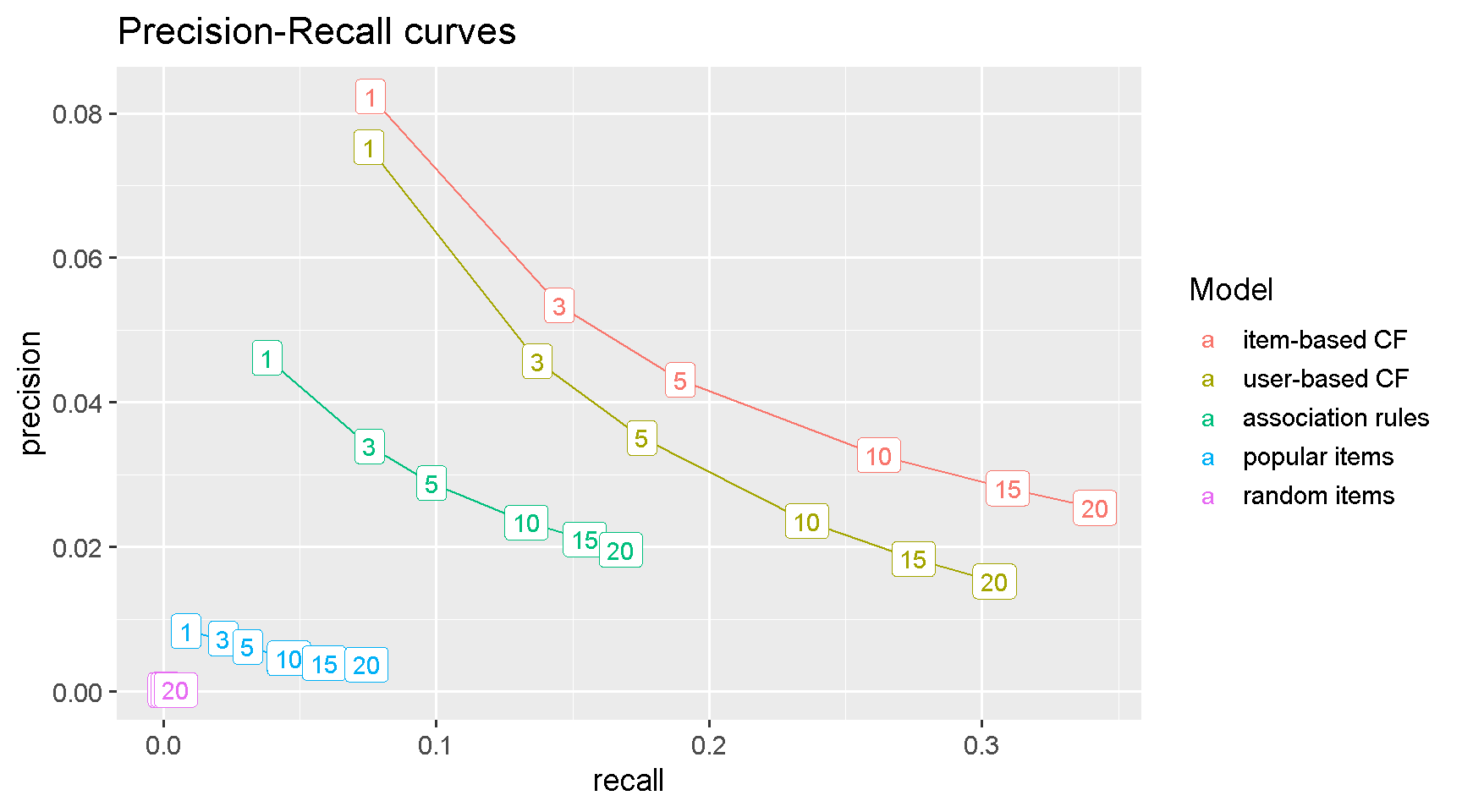
Precision-Recall curve
Another common way to compare the performance of classification models is with Precision Vs Recall curves. Precision shows how sensitive models are to False Positives (i.e. recommending an item not very likely to be purchased) whereas Recall (which is just another name for the TPR) looks at how sensitive models are to False Negatives (i.e. do not suggest an item which is highly likely to be purchased).
Normally, we care about accurately predicting which items are more likely to be purchased because this would have a positive impact on sales and revenue. In other words, we want to maximise Recall (or minimise FNs) for the same Precision.
The plot confirms that item-based CF is the best model because it has higher Recall (i.e. lower FNs) for any given level of Precision. This means that IBCF minimises FNs (i.e. not suggesting an item highly likely to be purchased) for all level of FPs.
results_tbl %>%
ggplot(aes(recall, precision,
colour = fct_reorder2(as.factor(name), precision, recall))) +
geom_line() +
geom_label(aes(label = n)) +
labs(title = "Precision-Recall curves",
colour = "Model") +
theme_grey(base_size = 14)
Predictions for a new user
The final step is to generate a prediction with the best performing model. To do that, I need to create a made-up purchase order.
First, I create a string containing 6 products selected at random.
customer_order <- c("GREEN REGENCY TEACUP AND SAUCER",
"SET OF 3 BUTTERFLY COOKIE CUTTERS",
"JAM MAKING SET WITH JARS",
"SET OF TEA COFFEE SUGAR TINS PANTRY",
"SET OF 4 PANTRY JELLY MOULDS")
Next, I put this order in a format that recommenderlab accepts.
new_order_rat_matrx <- retail %>%
# Select item descriptions from retail dataset
select(Description) %>%
unique() %>%
# Add a 'value' column with 1's for customer order items
mutate(value = as.numeric(Description %in% customer_order)) %>%
# Spread into sparse matrix format
spread(key = Description, value = value) %>%
# Change to a matrix
as.matrix() %>%
# Convert to recommenderlab class 'binaryRatingsMatrix'
as("binaryRatingMatrix")
Now, I can create a Recommender. I use getData to retrieve training data and set method = “IBCF” to select the best performing model (“item-based collaborative filtering”).
recomm <- Recommender(getData(scheme, 'train'),
method = "IBCF",
param = list(k = 5))
recomm
## Recommender of type 'IBCF' for 'binaryRatingMatrix'
## learned using 15832 users.
Finally, I can pass the Recommender and the made-up order to the predict function to create a top 10 recommendation list for the new customer.
pred <- predict(recomm,
newdata = new_order_rat_matrx,
n = 10)
Lastly, the suggested items can be inspected as a list.
as(pred, 'list')
## $`1`
## [1] "ROSES REGENCY TEACUP AND SAUCER"
## [2] "PINK REGENCY TEACUP AND SAUCER"
## [3] "SET OF 3 HEART COOKIE CUTTERS"
## [4] "JAM MAKING SET PRINTED"
## [5] "REGENCY CAKESTAND 3 TIER"
## [6] "SET OF 3 CAKE TINS PANTRY DESIGN"
## [7] "GINGERBREAD MAN COOKIE CUTTER"
## [8] "SET OF 3 REGENCY CAKE TINS"
## [9] "RECIPE BOX PANTRY YELLOW DESIGN"
## [10] "3 PIECE SPACEBOY COOKIE CUTTER SET"
Comments
This brings to an end the modelling and evaluation part of this project, which I found straightforward and quite enjoyable. recommenderlab is intuitive and easy to use and I particularly appreciated its ability to estimate and compare several classification algorithms at the same time. In summary, I have learned how to carry out Market Basket Analysis with recommenderlab in R, how to interpret the results and choose the best performing model.
Code Repository
The full R code can be found on my GitHub profile
References
- For Recommenderlab Package see: https://cran.r-project.org/package=recommenderlab
- For Recommenderlab Package Vignette see: https://cran.r-project.org/web/packages/recommenderlab/vignettes/recommenderlab.pdf